2.2.2: Initial Value Problem of Cauchy

Consider again the quasilinear equation

(\(\star\)) \(a_1(x,y,u)u_x+a_2(x,y,u)u_y=a_3(x,y,u)\).

Let
$$
\Gamma:\ \ x=x_0(s),\ y=y_0(s),\ z=z_0(s), \ s_1\le s\le s_2,\ -\infty<s_1<s_2<+\infty
$$
be a regular curve in \(\mathbb{R}^3\) and denote by \(\mathcal{C}\) the orthogonal projection of \(\Gamma\) onto the \((x,y)\)-plane, i. e.,
$$
\mathcal{C}:\ \ x=x_0(s),\ \ y=y_0(s).
\]

Initial value problem of Cauchy: Find a \(C^1\)-solution \(u=u(x,y)\) of \((\star)\) such that \(u(x_0(s),y_0(s))=z_0(s)\), i. e., we seek a surface \(\mathcal{S}\) defined by \(z=u(x,y)\) which contains the curve \(\Gamma\).

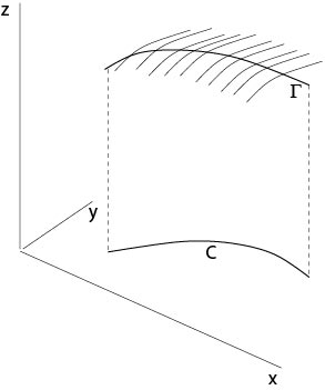
Figure 2.2.2.1: Cauchy initial value problem

Definition. The curve \(\Gamma\) is said to be non-characteristic if
$$
x_0'(s)a_2(x_0(s),y_0(s))-y_0'(s)a_1(x_0(s),y_0(s))\not=0.
\]

Theorem 2.1. Assume \(a_1,\ a_2,\ a_2\in C^1\) in their arguments, the initial data \(x_0,\ y_0,\ z_0\in C^1[s_1,s_2]\) and \(\Gamma\) is non-characteristic.

Then there is a neighborhood of \(\cal{C}\) such that there exists exactly one solution \(u\) of the Cauchy initial value problem.

Proof. (i) Existence. Consider the following initial value problem for the system of characteristic equations to (\(\star\)):
\begin{eqnarray*}
x'(t)&=&a_1(x,y,z)\\
y'(t)&=&a_2(x,y,z)\\
z'(t)&=&a_3(x,y,z)
\end{eqnarray*}
with the initial conditions
\begin{eqnarray*}
x(s,0)&=&x_0(s)\\
y(s,0)&=&y_0(s)\\
z(s,0)&=&z_0(s).
\end{eqnarray*}
Let \(x=x(s,t)\), \(y=y(s,t)\), \(z=z(s,t)\) be the solution, \(s_1\le s\le s_2\), \(|t|<\eta\) for an \(\eta>0\). We will show that this set of curves, see Figure 2.2.2.1, defines a surface. To show this, we consider the inverse functions \(s=s(x,y)\), \(t=t(x,y)\) of \(x=x(s,t)\), \(y=y(s,t)\) and show that \(z(s(x,y),t(x,y))\) is a solution of the initial problem of Cauchy. The inverse functions \(s\) and \(t\) exist in a neighborhood of \(t=0\) since
$$
\det \frac{\partial(x,y)}{\partial(s,t)}\Big|_{t=0}=
\left|\begin{array}{cc}x_s&x_t\\y_s&y_t\end{array}\right|_{t=0}
=x_0'(s)a_2-y_0'(s)a_1\not=0,
$$
and the initial curve \(\Gamma\) is non-characteristic by assumption.

Set
$$
u(x,y):=z(s(x,y),t(x,y)),
$$
then \(u\) satisfies the initial condition since
$$
u(x,y)|_{t=0}=z(s,0)=z_0(s).
$$
The following calculation shows that \(u\) is also a solution of the differential equation (\(\star\)).
\begin{eqnarray*}
a_1u_x+a_2u_y&=&a_1(z_ss_x+z_tt_x)+a_2(z_ss_y+z_tt_y)\\
&=&z_s(a_1s_x+a_2s_y)+z_t(a_1t_x+a_2t_y)\\
&=&z_s(s_xx_t+s_yy_t)+z_t(t_xx_t+t_yy_t)\\
&=&a_3
\end{eqnarray*}
since \(0=s_t=s_xx_t+s_yy_t\) and \(1=t_t=t_xx_t+t_yy_t\).

(ii) Uniqueness. Suppose that \(v(x,y)\) is a second solution. Consider a point \((x',y')\) in a neighborhood of the curve \((x_0(s),y(s))\), \(s_1-\epsilon\le s\le s_2+\epsilon\), \(\epsilon>0\) small. The inverse parameters are \(s'=s(x',y')\), \(t'=t(x',y')\), see Figure 2.2.2.2.

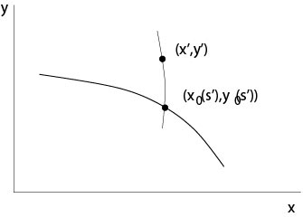
Figure 2.2.2.2: Uniqueness proof

Let
$$
{\mathcal{A}}:\ \ x(t):=x(s',t),\ y(t):=y(s',t),\ z(t):=z(s',t)
$$
be the solution of the above initial value problem for the characteristic differential equations with the initial data
$$
x(s',0)=x_0(s'),\ y(s',0)=y_0(s'),\ z(s',0)=z_0(s').
$$
According to its construction this curve is on the surface \(\mathcal{S}\) defined by \(u=u(x,y)\) and \(u(x',y')=z(s',t')\). Set
$$
\psi(t):=v(x(t),y(t))-z(t),
$$
then
\begin{eqnarray*}
\psi'(t)&=&v_xx'+v_yy'-z'\\
&=&x_xa_1+v_ya_2-a_3=0
\end{eqnarray*}
and
$$
\psi(0)=v(x(s',0),y(s',0))-z(s',0) =0
$$
since \(v\) is a solution of the differential equation and satisfies the initial condition by assumption. Thus, \(\psi(t)\equiv0\), i. e.,
$$
v(x(s',t),y(s',t))-z(s',t)=0.
$$
Set \(t=t'\), then
$$
v(x',y')-z(s',t')=0,
$$
which shows that \(v(x',y')=u(x',y')\) because of \(z(s',t')=u(x',y')\).

\(\Box\)

Remark. In general, there is no uniqueness if the initial curve \(\Gamma\) is a characteristic curve, see an exercise and Figure 2.2.2.3, which illustrates this case.

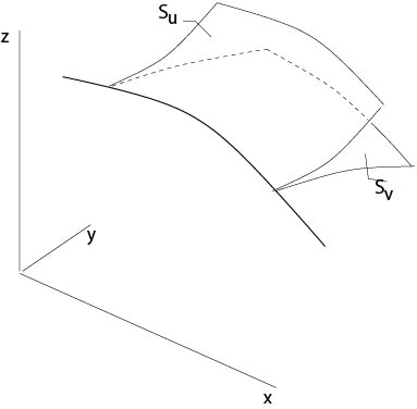
Figure 2.2.2.3: Multiple solutions

Examples

Example 2.2.2.1:

Consider the Cauchy initial value problem
$$
u_x+u_y=0
$$
with the initial data
$$
x_0(s)=s,\ y_0(s)=1,\ z_0(s)\ \mbox{is a given}\ C^1\mbox{-function}.
$$
These initial data are non-characteristic since \(y_0'a_1-x_0'a_2=-1\). The solution of the associated system of characteristic equations
$$
x'(t)=1,\ y'(t)=1,\ u'(t)=0
$$
with the initial conditions
$$
x(s,0)=x_0(s),\ y(s,0)=y_0(s),\ z(s,0)=z_0(s)
$$
is given by
$$
x=t+x_0(s),\ y=t+y_0(s),\ z=z_0(s) ,
$$
i. e.,
$$
x=t+s,\ y=t+1,\ z=z_0(s).
$$
It follows \(s=x-y+1,\ t=y-1\) and that \(u=z_0(x-y+1)\) is the solution of the Cauchy initial value problem.

Example 2.2.2.2:

A problem from kinetics in chemistry. Consider for \(x\ge0\), \(y\ge0\) the problem
$$
u_x+u_y=\left(k_0e^{-k_1x}+k_2\right)(1-u)
$$
with initial data
$$
u(x,0)=0,\ x>0,\ \mbox{and}\ u(0,y)=u_0(y),\ y>0.
$$
Here the constants \(k_j\) are positive, these constants define the velocity of the reactions in consideration, and the function \(u_0(y)\) is given. The variable \(x\) is the time and \(y\) is the height of a tube, for example, in which the chemical reaction takes place, and \(u\) is the concentration of the chemical substance.

In contrast to our previous assumptions, the initial data are not in \(C^1\). The projection \({\mathcal C}_1\cup {\mathcal C}_2\) of the initial curve onto the \((x,y)\)-plane has a corner at the origin, see Figure 2.2.2.4.

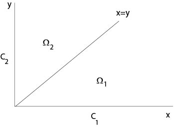
Figure 2.2.2.4: Domains to the chemical kinetics example

The associated system of characteristic equations is
$$
x'(t)=1,\ y'(t)=1,\ z'(t)=\left(k_0e^{-k_1x}+k_2\right)(1-z).
$$
It follows \(x=t+c_1\), \(y=t+c_2\) with constants \(c_j\). Thus the projection of the characteristic curves on the \((x,y)\)-plane are straight lines parallel to \(y=x\). We will solve the initial value problems in the domains \(\Omega_1\) and \(\Omega_2\), see Figure 2.2.2.4, separately.

(i) The initial value problem in \(\Omega_1\). The initial data are
$$
x_0(s)=s,\ y_0(s)=0, \ z_0(0)=0,\ s\ge 0.
$$
It follows
$$
x=x(s,t)=t+s,\ y=y(s,t)=t.
$$
Thus
$$
z'(t)=(k_0e^{-k_1(t+s)}+k_2)(1-z),\ z(0)=0.
$$
The solution of this initial value problem is given by
$$
z(s,t)=1-\exp\left(\frac{k_0}{k_1}e^{-k_1(s+t)}-k_2t-\frac{k_0}{k_1}e^{-k_1s}\right).
$$
Consequently
$$
u_1(x,y)=1-\exp\left(\frac{k_0}{k_1}e^{-k_1x}-k_2y-{k_0}{k_1}e^{-k_1(x-y)}\right)
$$
is the solution of the Cauchy initial value problem in \(\Omega_1\). If time \(x\) tends to \(\infty\), we get the limit
$$
\lim_{x\to\infty} u_1(x,y)=1-e^{-k_2y}.
\]

(ii) The initial value problem in \(\Omega_2\). The initial data are here

$$
x_0(s)=0,\ y_0(s)=s, \ z_0(0)=u_0(s),\ s\ge 0.
$$
It follows
$$
x=x(s,t)=t,\ y=y(s,t)=t+s.
$$
Thus
$$
z'(t)=(k_0e^{-k_1t}+k_2)(1-z),\ z(0)=0.
$$
The solution of this initial value problem is given by
$$
z(s,t)=1-(1-u_0(s))\exp\left(\frac{k_0}{k_1}e^{-k_1t}-k_2t-\frac{k_0}{k_1}\right).
$$
Consequently
$$
u_2(x,y)=1-(1-u_0(y-x))\exp\left(\frac{k_0}{k_1}e^{-k_1x}-k_2x-\frac{k_0}{k_1}\right)
$$
is the solution in \(\Omega_2\).

If \(x=y\), then
\begin{eqnarray*}
u_1(x,y)&=&1-\exp\left(\frac{k_0}{k_1}e^{-k_1x}-k_2x-\frac{k_0}{k_1}\right)\\
u_2(x,y)&=&1-(1-u_0(0))\exp\left(\frac{k_0}{k_1}e^{-k_1x}-k_2x-\frac{k_0}{k_1}\right).
\end{eqnarray*}
If \(u_0(0)>0\), then \(u_1<u_2\) if \(x=y\), i. e., there is a jump of the concentration of the substrate along its burning front defined by \(x=y\).

Remark. Such a problem with discontinuous initial data is called Riemann problem. See an exercise for another Riemann problem.

The case that a solution of the equation is known

Here we will see that we get immediately a solution of the Cauchy initial value problem if a solution of the homogeneous linear equation
$$
a_1(x,y)u_x+a_2(x,y)u_y=0
$$
is known.

Let
$$
x_0(s),\ y_0(s),\ z_0(s),\ s_1<s<s_2
$$
be the initial data and let \(u=\phi(x,y)\) be a solution of the differential equation. We assume that
$$
\phi_x(x_0(s),y_0(s))x_0'(s)+\phi_y(x_0(s),y_0(s))y_0'(s)\not=0
$$
is satisfied. Set
$$
g(s)=\phi(x_0(s),y_0(s))
$$
and let \(s=h(g)\) be the inverse function.

The solution of the Cauchy initial problem is given by \(u_0\left(h(\phi(x,y))\right)\).

This follows since in the problem considered a composition of a solution is a solution again, see an exercise, and since
$$
u_0\left(h(\phi(x_0(s),y_0(s))\right)=u_0(h(g))=u_0(s).
\]

Example 2.2.2.3:

Consider equation
$$
u_x+u_y=0
$$
with initial data
$$
x_0(s)=s,\ y_0(s)=1,\ u_0(s)\ \mbox{is a given function}.
$$
A solution of the differential equation is \(\phi(x,y)=x-y\). Thus
$$
\phi((x_0(s),y_0(s))=s-1
$$
and
$$
u_0(\phi+1)=u_0(x-y+1)
$$
is the solution of the problem.

Contributors and Attributions

• Prof. Dr. Erich Miersemann (Universität Leipzig)

• Integrated by Justin Marshall.