
3.1: Linear Systems with Two Variables and Their Solutions
- Page ID
- 6240
Learning Objectives
- Check solutions to systems of linear equations.
- Solve linear systems using the graphing method.
- Identify a dependent and inconsistent systems.
Definition of a Linear System with Two Variable
Real-world applications are often modeled using more than one variable and more than one equation. A system of equations1 consists of a set of two or more equations with the same variables. In this section, we will study linear systems2 consisting of two linear equations each with two variables. For example,
\(\left\{ \begin{array} { l } { 2 x - 3 y = 0 } \\ { - 4 x + 2 y = - 8 } \end{array} \right.\)
A solution to a linear system3, or simultaneous solution4, is an ordered pair \((x, y)\) that solves both of the equations. In this case, \((3, 2)\) is the only solution. To check that an ordered pair is a solution, substitute the corresponding \(x\)- and \(y\)-values into each equation and then simplify to see if you obtain a true statement for both equations.
| Check: \((3, 2)\) | |
| Equation 1: \(2 x - 3 y = 0\) | Equation 2: \(- 4 x + 2 y = - 8\) |
| \(\begin{aligned} 2 ( \color{Cerulean}{3}\color{Black}{ ) }- 3 ( \color{Cerulean}{2}\color{Black}{ )} & = 0 \\ 6 - 6 & = 0 \\ 0 & = 0 \color{Cerulean}{✓} \end{aligned}\) | \(\begin{aligned} - 4 ( \color{Cerulean}{3}\color{Black}{ )} + 2 ( \color{Cerulean}{2}\color{Black}{ )} & = - 8 \\ - 12 + 4 & = - 8 \\ - 8 & = - 8 \color{Cerulean}{✓}\end{aligned}\) |
Example \(\PageIndex{1}\):
Determine whether or not \((1,0)\) is a solution to the system \(\left\{ \begin{array} { c } { x - y = 1 } \\ { - 2 x + 3 y = 5 } \end{array} \right.\).
Solution
Substitute the appropriate values into both equations.
| Check: \((1, 0)\) | |
| Equation 1: \(x - y = 1\) | Equation 2: \(- 2 x + 3 y = 5\) |
| \(\begin{aligned} ( \color{Cerulean}{1}\color{Black}{ )} - ( \color{Cerulean}{0}\color{Black}{ )} & = 1 \\ 1 - 0 & = 1 \\ 1 & = 1 \color{Cerulean}{✓} \end{aligned}\) | \(\begin{array} { r } { - 2 ( \color{Cerulean}{1}\color{Black}{ )} + 3 ( \color{Cerulean}{0}\color{Black}{ )} = 5 } \\ { - 2 + 0 = 5 } \\ { - 2 = 5 } \color{red}{✗} \end{array}\) |
Answer:
Since \((1, 0)\) does not satisfy both equations, it is not a solution.
Exercise \(\PageIndex{1}\)
Is \((-2, 4)\) a solution to the system \(\left\{ \begin{array} { c } { x - y = - 6 } \\ { - 2 x + 3 y = 16 } \end{array} \right. \)?
- Answer
-
Yes
www.youtube.com/v/VBCsv2IsjBk
Solve by Graphing
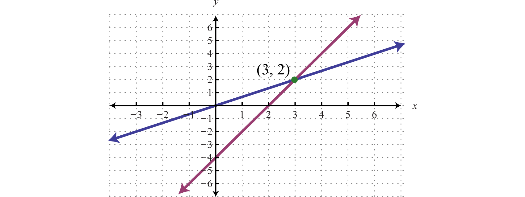
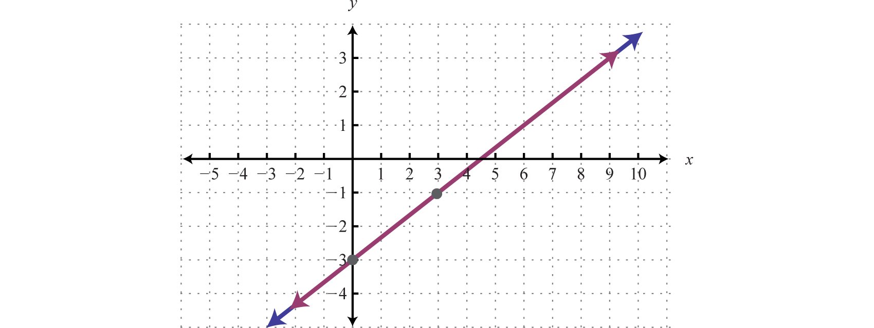
Geometrically, a linear system consists of two lines, where a solution is a point of intersection. To illustrate this, we will graph the following linear system with a solution of \((3, 2)\):
\(\left\{ \begin{array} { c } { 2 x - 3 y = 0 } \\ { - 4 x + 2 y = - 8 } \end{array} \right.\)
First, rewrite the equations in slope-intercept form so that we may easily graph them.
| \(\begin{aligned} 2 x - 3 y & = 0 \\ 2 x - 3 y \color{Cerulean}{- 2 x} & \color{Black}{=} 0 \color{Cerulean}{- 2 x} \\ - 3 y & = - 2 x \\ \frac { - 3 y } { \color{Cerulean}{- 3} } & = \frac { - 2 x } { \color{Cerulean}{- 3} } \\ y & = \frac { 2 } { 3 } x \end{aligned}\) | \(\begin{aligned} - 4 x + 2 y & = - 8 \\ - 4 x + 2 y \color{Cerulean}{+ 4 x} & \color{Black}{=} - 8 \color{Cerulean}{+ 4 x} \\ 2 y & = 4 x - 8 \\ \frac { 2 y } { \color{Cerulean}{2} } & \color{Black}{=} \frac { 4 x - 8 } { \color{Cerulean}{2} } \\ y & = 2 x - 4 \end{aligned}\) |
Next, replace these forms of the original equations in the system to obtain what is called an equivalent system5. Equivalent systems share the same solution set.
\(\begin{array} { c } { \color {Cerulean} { Original\: system } \:\:\:\:\:\:\:\color{Cerulean}{Equivalent\: system}} \\ { \left\{ \begin{array} { c } { 2 x - 3 y = 0 } \\ { - 4 x + 2 y = - 8 } \end{array} \right. \:\:\:\Rightarrow \:\:\:\:\:\left\{ \begin{array} { l } { y = \frac { 2 } { 3 } x } \\ { y = 2 x - 4 } \end{array} \right. } \end{array}\)
If we graph both of the lines on the same set of axes, then we can see that the point of intersection is indeed \((3, 2)\), the solution to the system.
To summarize, linear systems described in this section consist of two linear equations each with two variables. A solution is an ordered pair that corresponds to a point where the two lines intersect in the rectangular coordinate plane. Therefore, one way to solve linear systems is by graphing both lines on the same set of axes and determining the point where they cross. This describes the graphing method6 for solving linear systems.
When graphing the lines, take care to choose a good scale and use a straightedge to draw the line through the points; accuracy is very important here.
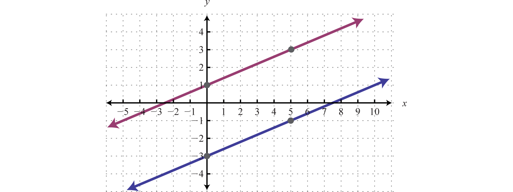
Example \(\PageIndex{2}\):
Solve by graphing: \(\left\{ \begin{array} { l } { x - y = - 4 } \\ { 2 x + y = 1 } \end{array} \right.\).
Solution
Rewrite the linear equations in slope-intercept form.
| \(\begin{aligned} x - y & = - 4 \\ - y & = - x - 4 \\ \frac { - y } { \color{Cerulean}{- 1} } & \color{Black}{=} \frac { - x - 4 } { \color{Cerulean}{- 1} } \\ y & = x + 4 \end{aligned}\) | \(\begin{aligned} 2 x + y & = 1 \\ y & = - 2 x + 1 \end{aligned}\) |
Write the equivalent system and graph the lines on the same set of axes.
\(\left\{ \begin{array} { l } { x - y = - 4 } \\ { 2 x + y = 1 } \end{array} \right. \Rightarrow \left\{ \begin{array} { l } { y = x + 4 } \\ { y = - 2 x + 1 } \end{array} \right.\)
|
\(\color{Cerulean}{Line 1:} y=x+4\) \(y-intercept: (0,4)\) \(slope: m = 1 = \frac{1}{1} = \frac{rise}{run}\) |
\(\color{Cerulean}{Line 2:} y=-2x+1\) \(y-intercept: (0,1)\) \(slope: m=-2 = frac{-2}{1} = \frac{rise}{run}\) |
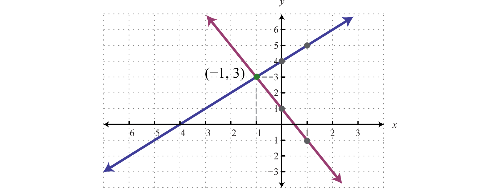
Use the graph to estimate the point where the lines intersect and check to see if it solves the original system. In the above graph, the point of intersection appears to be \((−1, 3)\).
| Check: \((-1, 3)\) | |
| Line 1: \(x-y=-4\) | Line 2: \(2x+y=1\) |
| \(\begin{array} { r } { ( \color{Cerulean}{- 1} \color{Black}{)} - ( \color{Cerulean}{3} \color{Black}{)} = - 4 } \\ { - 1 - 3 = - 4 } \\ { - 4 = - 4 } \end{array}\color{Cerulean}{✓}\) | \(\begin{array} { r } { 2 ( \color{Cerulean}{- 1} \color{Black}{)} + ( \color{Cerulean}{3} \color{Black}{)} = 1 } \\ { - 2 + 3 = 1 } \\ { 1 = 1 } \end{array}\color{Cerulean}{✓}\) |
Answer:
\((-1, 3)\)
Example \(\PageIndex{3}\):
Solve by graphing: \(\left\{ \begin{array} { c } { 2 x + y = 2 } \\ { - 2 x + 3 y = - 18 } \end{array} \right.\).
Solution
We first solve each equation for \(y\) to obtain an equivalent system where the lines are in slope-intercept form.
\(\left\{ \begin{array} { c c } { 2 x + y = 2 } \\ { - 2 x + 3 y = - 18 } \end{array} \right. \Rightarrow \left\{ \begin{array} { l } { y = - 2 x + 2 } \\ { y = \frac { 2 } { 3 } x - 6 } \end{array} \right.\)
Graph the lines and determine the point of intersection.
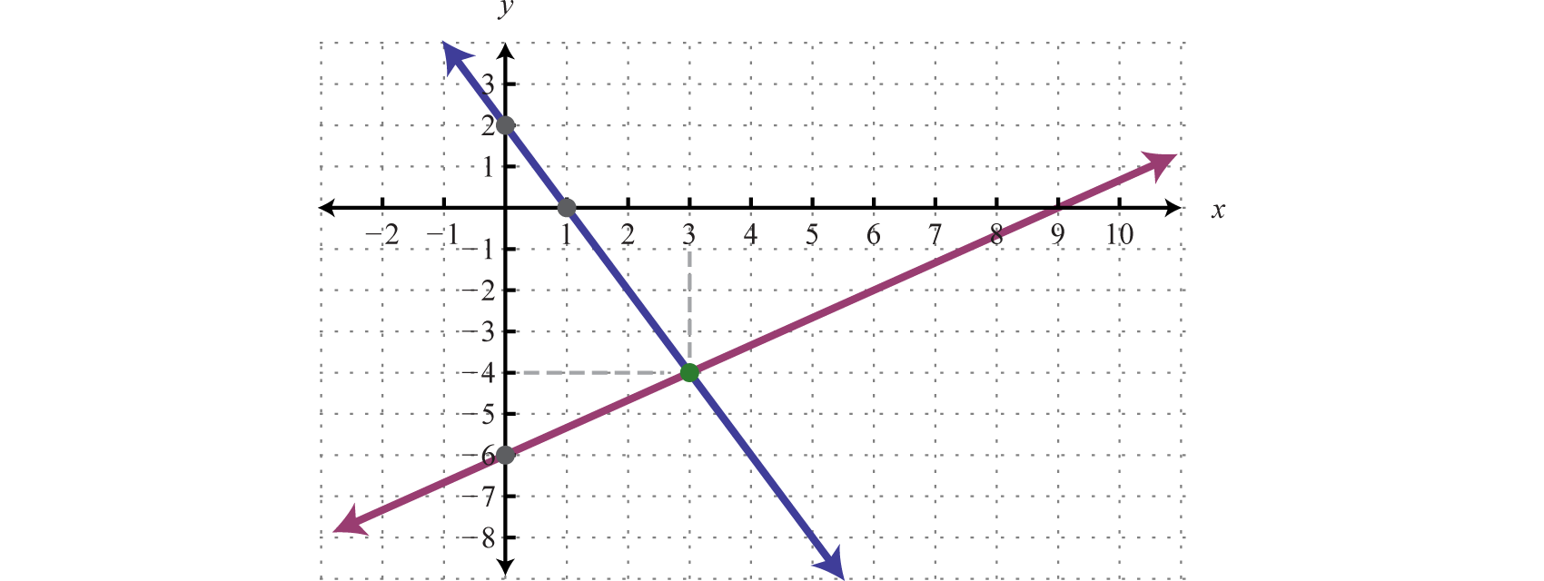
| Check: \((3, -4)\) | |
| \(\begin{array} { r } { 2 x + y = 2 } \\ { 2 ( \color{Cerulean}{3}\color{Black}{ )} + ( \color{Cerulean}{- 4} \color{Black}{)} = 2 } \\ { 6 - 4 = 2 } \\ { 2 = 2 } \color{Cerulean}{✓} \end{array}\) | \(\begin{aligned} - 2 x + 3 y & = - 18 \\ - 2 ( \color{Cerulean}{3} \color{Black}{)} + 3 ( \color{Cerulean}{- 4} \color{Black}{)} & = - 18 \\ - 6 - 12 & = - 18 \\ - 18 & = - 18 \color{Cerulean}{✓}\end{aligned}\) |
Answer:
\((3, -4)\)
Example \(\PageIndex{4}\):
Solve by graphing: \(\left\{ \begin{array} { c } { 3 x + y = 6 } \\ { y = - 3 } \end{array} \right.\).
Solution
\(\left\{ \begin{array} { c } { 3 x + y = 6 } \\ { y = - 3 } \end{array} \right. \Rightarrow \left\{ \begin{array} { l } { y = - 3 x + 6 } \\ { y = - 3 } \end{array} \right.\)
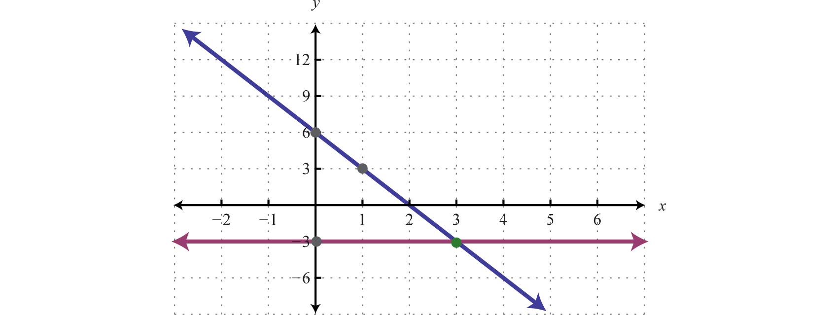
| Check: \((3, -3)\) | |
| \(\begin{array} { r } { 3 x + y = 6 } \\ { 3 ( \color{Cerulean}{3} \color{Black}{)} + ( \color{Cerulean}{- 3}\color{Black}{ )} = 6 } \\ { 9 - 3 = 6 } \\ { 6 = 6 } \color{Cerulean}{✓} \end{array}\) | \(\begin{aligned} y & = - 3 \\ ( \color{Cerulean}{- 3} \color{Black}{)} & = - 3 \\ - 3 & = - 3 \color{Cerulean}{✓} \end{aligned}\) |
Answer:
\((3, -3)\)
The graphing method for solving linear systems is not ideal when a solution consists of coordinates that are not integers. There will be more accurate algebraic methods in sections to come, but for now, the goal is to understand the geometry involved when solving systems. It is important to remember that the solutions to a system correspond to the point, or points, where the graphs of the equations intersect.
Exercise \(\PageIndex{2}\)
Solve by graphing: \(\left\{ \begin{array} { l } { - x + y = 6 } \\ { 5 x + 2 y = - 2 } \end{array} \right.\).
- Answer
-
\((-2, 4)\)
www.youtube.com/v/FMc7WVumxv0
Dependent and Inconsistent Systems
A system with at least one solution is called a consistent system7. Up to this point, all of the examples have been of consistent systems with exactly one ordered pair solution. It turns out that this is not always the case. Sometimes systems consist of two linear equations that are equivalent. If this is the case, the two lines are the same and when graphed will coincide. Hence, the solution set consists of all the points on the line. This is a dependent system8. Given a consistent linear system with two variables, there are two possible results:

A solution to an independent system9 is an ordered pair \((x, y)\). The solution to a dependent system consists of infinitely many ordered pairs \((x, y)\). Since any line can be written in slope-intercept form, \(y = mx + b\), we can express these solutions, dependent on \(x\), as follows:
\(\begin{array} { c } { \{ ( x , y ) | y = m x + b \} \:\:\:\color{Cerulean} { Set-Notation } } \\ { ( x , m x + b ) \quad \color{Cerulean} { Shortened\: Form } } \end{array}\)
In this text we will express all the ordered pair solutions \((x, y)\) in the shortened form \((x, mx + b)\), where \(x\) is any real number.
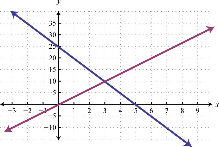
Example \(\PageIndex{5}\):
Solve by graphing: \(\left\{ \begin{array} { r } { - 2 x + 3 y = - 9 } \\ { 4 x - 6 y = 18 } \end{array} \right.\).
Solution
Determine slope-intercept form for each linear equation in the system.
| \(\begin{aligned} - 2 x + 3 y & = - 9 \\ - 2 x + 3 y & = - 9 \\ 3 y & = 2 x - 9 \\ y & = \frac { 2 x - 9 } { 3 } \\ y & = \frac { 2 } { 3 } x - 3 \end{aligned}\) | \(\begin{aligned} 4 x - 6 y & = 18 \\ 4 x - 6 y & = 18 \\ - 6 y & = - 4 x + 18 \\ y & = \frac { - 4 x + 18 } { - 6 } \\ y & = \frac { 2 } { 3 } x - 3 \end{aligned}\) |
\(\left\{ \begin{array} { c c } { - 2 x + 3 y = - 9 } \\ { 4 x - 6 y = 18 } \end{array} \right. \Rightarrow \left\{ \begin{array} { l } { y = \frac { 2 } { 3 } x - 3 } \\ { y = \frac { 2 } { 3 } x - 3 } \end{array} \right.\)
In slope-intercept form, we can easily see that the system consists of two lines with the same slope and same \(y\)-intercept. They are, in fact, the same line. And the system is dependent.
Answer:
\(\left( x , \frac { 2 } { 3 } x - 3 \right)\)
In this example, it is important to notice that the two lines have the same slope and same \(y\)-intercept. This tells us that the two equations are equivalent and that the simultaneous solutions are all the points on the line \(y = \frac{2}{3} x − 3\). This is a dependent system, and the infinitely many solutions are expressed using the form \((x, mx + b)\). Other resources may express this set using set notation, \(\{(x, y) | y = \frac{2}{3} x − 3\}\), which reads “the set of all ordered pairs \((x, y)\) such that \(y = \frac{2}{3} x − 3\).”
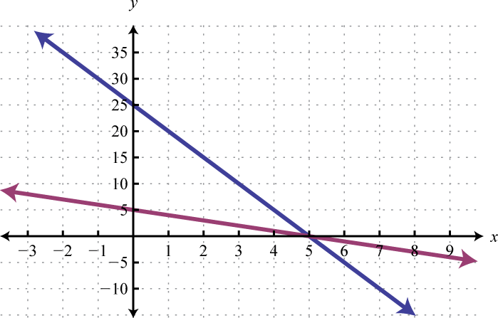
Sometimes the lines do not cross and there is no point of intersection. Such a system has no solution, \(Ø\), and is called an inconsistent system10.

Example \(\PageIndex{6}\):
Solve by graphing: \(\left\{ \begin{array} { l } { - 2 x + 5 y = - 15 } \\ { - 4 x + 10 y = 10 } \end{array} \right.\).
Solution
Determine the slope-intercept form for each linear equation.
| \(\begin{aligned} - 2 x + 5 y & = - 15 \\ - 2 x + 5 y & = - 15 \\ 5 y & = 2 x - 15 \\ y & = \frac { 2 x - 15 } { 5 } \\ y & = \frac { 2 } { 5 } x - 3 \end{aligned}\) | \(\begin{aligned} - 4 x + 10 y & = 10 \\ - 4 x + 10 y & = 10 \\ 10 y & = 4 x + 10 \\ y & = \frac { 4 x + 10 } { 10 } \\ y & = \frac { 2 } { 5 } x + 1 \end{aligned}\) |
\(\left\{ \begin{array} { l } { - 2 x + 5 y = - 15 } \\ { - 4 x + 10 y = 10 } \end{array} \right. \Rightarrow \left\{ \begin{array} { l } { y = \frac { 2 } { 5 } x - 3 } \\ { y = \frac { 2 } { 5 } x + 1 } \end{array} \right.\)
In slope-intercept form, we can easily see that the system consists of two lines with the same slope and different \(y\)-intercepts. Therefore, the lines are parallel and will never intersect.
Answer:
There is no simultaneous solution \(\varnothing\).
Exercise \(\PageIndex{3}\)
Solve by graphing: \(\left\{ \begin{array} { c } { x + y = - 1 } \\ { - 2 x - 2 y = 2 } \end{array} \right.\).
- Answer
-
\(( x , - x - 1 )\)
www.youtube.com/v/MuQ2oqI7sAg
Key Takeaways
- In this section, we limit our study to systems of two linear equations with two variables. Solutions to such systems, if they exist, consist of ordered pairs that satisfy both equations. Geometrically, solutions are the points where the graphs intersect.
- The graphing method for solving linear systems requires us to graph both of the lines on the same set of axes as a means to determine where they intersect.
- The graphing method is not the most accurate method for determining solutions, particularly when a solution has coordinates that are not integers. It is a good practice to always check your solutions.
- Some linear systems have no simultaneous solution. These systems consist of equations that represent parallel lines with different \(y\)-intercepts and do not intersect in the plane. They are called inconsistent systems and the solution set is the empty set, \(Ø\).
- Some linear systems have infinitely many simultaneous solutions. These systems consist of equations that are equivalent and represent the same line. They are called dependent systems and their solutions are expressed using the notation \((x, mx + b)\), where \(x\) is any real number.
Exercise \(\PageIndex{4}\)
Determine whether or not the given ordered pair is a solution to the given system.
1. \((3, -2)\);
\(\left\{ \begin{array} { c } { x + y = - 1 } \\ { - 2 x - 2 y = 2 } \end{array} \right.\)
2. \((-5, 0)\);
\(\left\{ \begin{array} { l } { x + y = - 1 } \\ { - 2 x - 2 y = 2 } \end{array} \right.\)
3. \(( - 2 , - 6 )\);
\(\left\{ \begin{array} { l } { - x + y = - 4 } \\ { 3 x - y = - 12 } \end{array} \right.\)
4. \(( 2 , - 7 )\);
\(\left\{ \begin{array} { l } { 3 x + 2 y = - 8 } \\ { - 5 x - 3 y = 11 } \end{array} \right.\)
5. \(( 0 , - 3 )\);
\(\left\{ \begin{array} { l } { 5 x - 5 y = 15 } \\ { - 13 x + 2 y = - 6 } \end{array} \right.\)
6. \(\left( - \frac { 1 } { 2 } , \frac { 1 } { 4 } \right)\);
\(\left\{ \begin{array} { l } { x + y = - \frac { 1 } { 4 } } \\ { - 2 x - 4 y = 0 } \end{array} \right.\)
7. \(\left( \frac { 3 } { 4 } , \frac { 1 } { 4 } \right)\);
\(\left\{ \begin{array} { l } { - x - y = - 1 } \\ { - 4 x - 8 y = 5 } \end{array} \right.\)
8. \(( - 3,4 )\);
\(\left\{ \begin{array} { l } { \frac { 1 } { 3 } x + \frac { 1 } { 2 } y = 1 } \\ { \frac { 2 } { 3 } x - \frac { 3 } { 2 } y = - 8 } \end{array} \right.\)
9. \(( - 5 , - 3 )\);
\(\left\{ \begin{array} { c } { y = - 3 } \\ { 5 x - 10 y = 5 } \end{array} \right.\)
10. \(( 4,2 )\);
\(\left\{ \begin{aligned} x & = 4 \\ - 7 x + 4 y & = 8 \end{aligned} \right.\)
- Answer
-
1. No
3. No
5. Yes
7. No
9. Yes
Exercise \(\PageIndex{5}\)
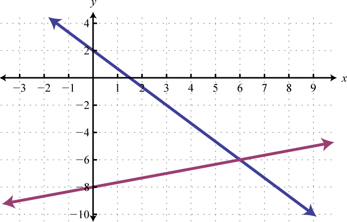
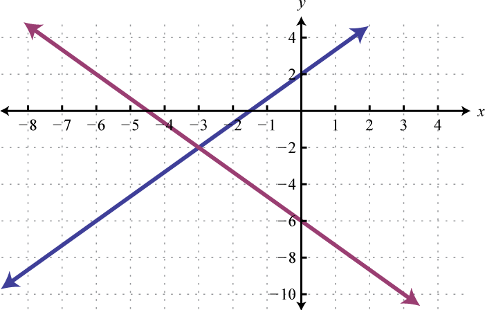
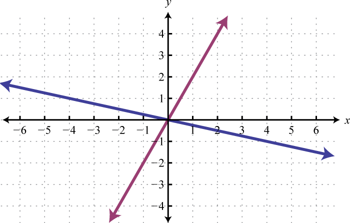
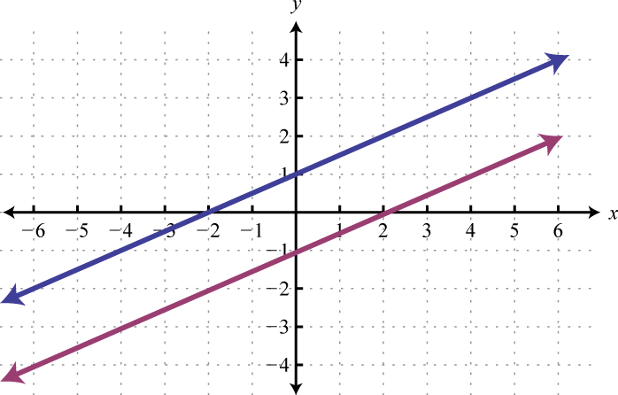
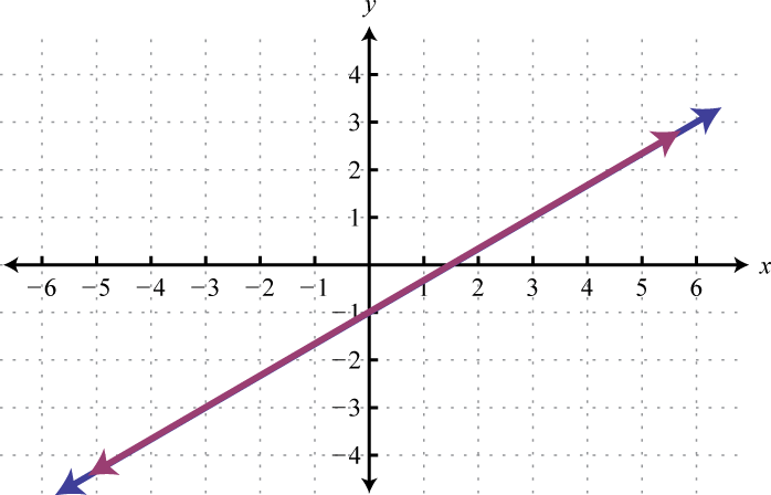
Given the graphs, determine the simultaneous solution.
2.
3.
4.
5.
6.
7.
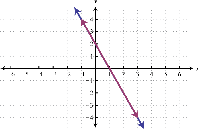
8.
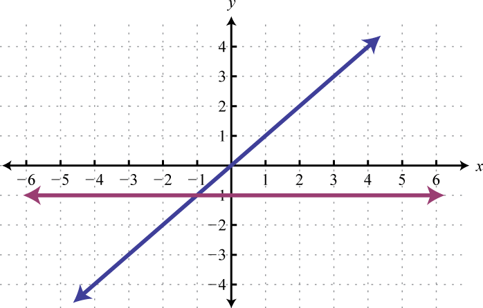
9.
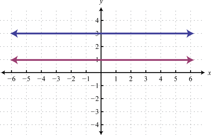
10.
- Answer
-
1. \((5, 0)\)
3. \((6, -6)\)
5. \((0,0)\)
7. \(( x , - 2 x + 2 )\)
9. \(\emptyset\)
Exercise \(\PageIndex{6}\)
Solve by graphing.
- \(\left\{ \begin{array} { l } { y = \frac { 3 } { 2 } x + 6 } \\ { y = - x + 1 } \end{array} \right.\)
- \(\left\{ \begin{array} { l } { y = \frac { 3 } { 4 } x + 2 } \\ { y = - \frac { 1 } { 4 } x - 2 } \end{array} \right.\)
- \(\left\{ \begin{array} { l } { y = x - 4 } \\ { y = - x + 2 } \end{array} \right.\)
- \(\left\{ \begin{array} { l } { y = - 5 x + 4 } \\ { y = 4 x - 5 } \end{array} \right.\)
- \(\left\{ \begin{array} { c } { y = \frac { 2 } { 5 } x + 1 } \\ { y = \frac { 3 } { 5 } x } \end{array} \right.\)
- \(\left\{ \begin{array} { l } { y = - \frac { 2 } { 5 } x + 6 } \\ { y = \frac { 2 } { 5 } x + 10 } \end{array} \right.\)
- \(\left\{ \begin{array} { l } { y = - 2 } \\ { y = x + 1 } \end{array} \right.\)
- \(\left\{ \begin{array} { l } { y = 3 } \\ { x = - 3 } \end{array} \right.\)
- \(\left\{ \begin{array} { l } { y = 0 } \\ { y = \frac { 2 } { 5 } x - 4 } \end{array} \right.\)
- \(\left\{ \begin{array} { l } { x = 2 } \\ { y = 3 x } \end{array} \right.\)
- \(\left\{ \begin{array} { l } { y = \frac { 3 } { 5 } x - 6 } \\ { y = \frac { 3 } { 5 } x - 3 } \end{array} \right.\)
- \(\left\{ \begin{array} { l } { y = - \frac { 1 } { 2 } x + 1 } \\ { y = - \frac { 1 } { 2 } x + 1 } \end{array} \right.\)
- \(\left\{ \begin{array} { l } { 2 x + 3 y = 18 } \\ { - 6 x + 3 y = - 6 } \end{array} \right.\)
- \(\left\{ \begin{aligned} - 3 x + 4 y & = 20 \\ 2 x + 8 y & = 8 \end{aligned} \right.\)
- \(\left\{ \begin{array} { l } { - 2 x + y = 1 } \\ { 2 x - 3 y = 9 } \end{array} \right.\)
- \(\left\{ \begin{array} { l } { x + 2 y = - 8 } \\ { 5 x + 4 y = - 4 } \end{array} \right.\)
- \(\left\{ \begin{array} { l } { 4 x + 6 y = 36 } \\ { 2 x - 3 y = 6 } \end{array} \right.\)
- \(\left\{ \begin{array} { l } { 2 x - 3 y = 18 } \\ { 6 x - 3 y = - 6 } \end{array} \right.\)
- \(\left\{ \begin{array} { l } { 3 x + 5 y = 30 } \\ { - 6 x - 10 y = - 10 } \end{array} \right.\)
- \(\left\{ \begin{array} { c } { - x + 3 y = 3 } \\ { 5 x - 15 y = - 15 } \end{array} \right.\)
- \(\left\{ \begin{array} { l } { x - y = 0 } \\ { - x + y = 0 } \end{array} \right.\)
- \(\left\{ \begin{array} { c } { y = x } \\ { y - x = 1 } \end{array} \right.\)
- \(\left\{ \begin{array} { c } { 3 x + 2 y = 0 } \\ { x = 2 } \end{array} \right.\)
- \(\left\{ \begin{array} { l } { 2 x + \frac { 1 } { 3 } y = \frac { 2 } { 3 } } \\ { - 3 x + \frac { 1 } { 2 } y = - 2 } \end{array} \right.\)
- \(\left\{ \begin{array} { l } { \frac { 1 } { 10 } x + \frac { 1 } { 5 } y = 2 } \\ { - \frac { 1 } { 5 } x + \frac { 1 } { 5 } y = - 1 } \end{array} \right.\)
- \(\left\{ \begin{array} { l } { \frac { 1 } { 3 } x - \frac { 1 } { 2 } y = 1 } \\ { \frac { 1 } { 3 } x + \frac { 1 } { 5 } y = 1 } \end{array} \right.\)
- \(\left\{ \begin{array} { l } { \frac { 1 } { 9 } x + \frac { 1 } { 6 } y = 0 } \\ { \frac { 1 } { 9 } x + \frac { 1 } { 4 } y = \frac { 1 } { 2 } } \end{array} \right.\)
- \(\left\{ \begin{array} { l } { \frac { 5 } { 16 } x - \frac { 1 } { 2 } y = 5 } \\ { - \frac { 5 } { 16 } x + \frac { 1 } { 2 } y = \frac { 5 } { 2 } } \end{array} \right.\)
- \(\left\{ \begin{array} { c } { \frac { 1 } { 6 } x - \frac { 1 } { 2 } y = \frac { 9 } { 2 } } \\ { - \frac { 1 } { 18 } x + \frac { 1 } { 6 } y = - \frac { 3 } { 2 } } \end{array} \right.\)
- \(\left\{ \begin{array} { l } { \frac { 1 } { 2 } x - \frac { 1 } { 4 } y = - \frac { 1 } { 2 } } \\ { \frac { 1 } { 3 } x - \frac { 1 } { 2 } y = 3 } \end{array} \right.\)
- \(\left\{ \begin{array} { l } { y = 4 } \\ { x = - 5 } \end{array} \right.\)
- \(\left\{ \begin{array} { l } { y = - 3 } \\ { x = 2 } \end{array} \right.\)
- \(\left\{ \begin{array} { l } { y = 0 } \\ { x = 0 } \end{array} \right.\)
- \(\left\{ \begin{array} { l } { y = - 2 } \\ { y = 3 } \end{array} \right.\)
- \(\left\{ \begin{array} { l } { y = 5 } \\ { y = - 5 } \end{array} \right.\)
- \(\left\{ \begin{aligned} y & = 2 \\ y - 2 & = 0 \end{aligned} \right.\)
- \(\left\{ \begin{array} { l } { x = - 5 } \\ { x = 1 } \end{array} \right.\)
- \(\left\{ \begin{array} { l } { y = x } \\ { x = 0 } \end{array} \right.\)
- \(\left\{ \begin{array} { l } { 4 x + 6 y = 3 } \\ { - x + y = - 2 } \end{array} \right.\)
- \(\left\{ \begin{array} { l } { - 2 x + 20 y = 20 } \\ { 3 x + 10 y = - 10 } \end{array} \right.\)
- Assuming \(m\) is nonzero solve the system: \(\left\{ \begin{array} { l } { y = m x + b } \\ { y = - m x + b } \end{array} \right.\)
- Assuming \(b\) is nonzero solve the system: \(\left\{ \begin{array} { l } { y = m x + b } \\ { y = m x - b } \end{array} \right.\)
- Find the equation of the line perpendicular to \(y = −2x + 4\) and passing through \((3, 3)\). Graph this line and the given line on the same set of axes and determine where they intersect.
- Find the equation of the line perpendicular to \(y − x = 2\) and passing through \((−5, 1)\). Graph this line and the given line on the same set of axes and determine where they intersect.
- Find the equation of the line perpendicular to \(y = −5\) and passing through \((2, −5)\). Graph both lines on the same set of axes.
- Find the equation of the line perpendicular to the \(y\)-axis and passing through the origin.
- Use the graph of \(y = −\frac{2}{3} x + 3\) to determine the \(x\)-value where \(y = −3\). Verify your answer using algebra.
- Use the graph of \(y = \frac{4}{5} x − 3\) to determine the \(x\)-value where \(y = 5\). Verify your answer using algebra.
- Answer
-
1. \((−2, 3)\)
3. \((3, −1)\)
5. \((5, 3)\)
7. \((−3, −2)\)
9. \((10, 0)\)
11. \(Ø\)
13. \((3, 4)\)
15. \((−3, −5)\)
17. \((6, 2)\)
19. \(Ø\)
21. \((x, x)\)
23. \((2, −3)\)
25. \((10, 5)\)
27. \((−9, 6)\)
29. \((x, \frac{1}{3} x − 9)\)
31. \((−5, 4)\)
33. \((0, 0)\)
35. \(Ø\)
37. \(Ø\)
39. \((\frac{3}{2} , −\frac{1}{2})\)
41. \((0, b)\)
43. \(y = \frac{1}{2} x + \frac{3}{2} ; (1, 2)\)
45. \(x = 2\)
47. \(x = 9\)
Exercise \(\PageIndex{7}\)
- Discuss the weaknesses of the graphing method for solving systems.
- Explain why the solution set to a dependent linear system is denoted by \((x, mx + b)\).
- Draw a picture of a dependent linear system as well as a picture of an inconsistent linear system. What would you need to determine the equations of the lines that you have drawn?
- Answer
-
1. Answer may vary
3. Answer may vary
Footnotes
1A set of two or more equations with the same variables.
2A set of two or more linear equations with the same variables.
3Given a linear system with two equations and two variables, a solution is an ordered pair that satisfies both equations and corresponds to a point of intersection.
4Used when referring to a solution of a system of equations.
5A system consisting of equivalent equations that share the same solution set.
6A means of solving a system by graphing the equations on the same set of axes and determining where they intersect.
7A system with at least one solution.
8A linear system with two variables that consists of equivalent equations. It has infinitely many ordered pair solutions, denoted by \((x, mx + b)\).
9A linear system with two variables that has exactly one ordered pair solution.
10A system with no simultaneous solution.