
7.2: Exponential Functions and Their Graphs
- Page ID
- 6276
Learning Objectives
- Identify and evaluate exponential functions.
- Sketch the graph of exponential functions and determine the domain and range.
- Identify and graph the natural exponential function.
- Apply the formulas for compound interest.
Exponential Functions
At this point in our study of algebra we begin to look at transcendental functions or functions that seem to “transcend” algebra. We have studied functions with variable bases and constant exponents such as \(x^{2}\) or \(y^{−3}\). In this section we explore functions with a constant base and variable exponents. Given a real number \(b > 0\) where \(b ≠ 1\) an exponential function5 has the form,
\(f(x)=b^{x} \quad \color{Cerulean}{Exponential\:Function}\)
For example, if the base \(b\) is equal to \(2\), then we have the exponential function defined by \(f (x) = 2^{x}\). Here we can see the exponent is the variable. Up to this point, rational exponents have been defined but irrational exponents have not. Consider \(2^{\sqrt{7}}\), where the exponent is an irrational number in the range,
\(2.64<\sqrt{7}<2.65\)
We can use these bounds to estimate \(2^{\sqrt{7}}\),
\(2^{2.64}<2^{\sqrt{7}}<2^{2.65}\)
\(6.23<2^{\sqrt{7}}<6.28\)
Using rational exponents in this manner, an approximation of \(2^{\sqrt{7}}\) can be obtained to any level of accuracy. On a calculator,
\(2^{\wedge} \sqrt{7} \approx 6.26\)
Therefore the domain of any exponential function consists of all real numbers \((−∞, ∞)\). Choose some values for \(x\) and then determine the corresponding \(y\)-values.
| \(x\) | \(y\) | \(f(x)=2^{x}\) | \(\color{Cerulean}{Solutions}\) |
|---|---|---|---|
| \(-2\) | \(\color{Cerulean}{\frac{1}{4}}\) | \(y=2^{-2}=\frac{1}{2^{2}}=\frac{1}{4}\) | \(\left(-2, \frac{1}{4}\right)\) |
| \(-1\) | \(\color{Cerulean}{\frac{1}{2}}\) | \(y=2^{-1}=\frac{1}{2^{1}}=\frac{1}{2}\) | \(\left(-1, \frac{1}{2}\right)\) |
| \(0\) | \(\color{Cerulean}{1} \) | \(y=2^{0}=1\) | \((0,1)\) |
| \(1\) | \(\color{Cerulean}{2}\) | \(y=2^{1}=2\) | \((1,2)\) |
| \(2\) | \(\color{Cerulean}{4}\) | \(y=2^{2}=4\) | \((2,4)\) |
| \(\sqrt{7}\) | \(\color{Cerulean}{6.26}\) | \(y=2^{\sqrt{7}} \approx 6.26\) | \((2.65,6.26)\) |
Because exponents are defined for any real number we can sketch the graph using a continuous curve through these given points:
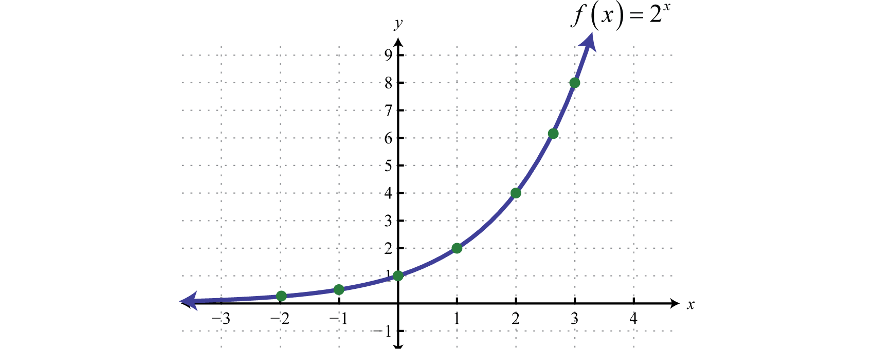
It is important to point out that as \(x\) approaches negative infinity, the results become very small but never actually attain zero. For example,
\(f(-5)=2^{-5}=\frac{1}{2^{5}} \approx 0.03125\)
\(f(-10)=2^{-10}=\frac{1}{2^{10}} \approx 0.0009766\)
\(f(-15)=2^{-15}=\frac{1}{2^{-15}} \approx .00003052\)
This describes a horizontal asymptote at \(y = 0\), the \(x\)-axis, and defines a lower bound for the range of the function: \((0, ∞)\).
The base \(b\) of an exponential function affects the rate at which it grows. Below we have graphed \(y = 2^{x} , y = 3^{x}\), and \(y = 10^{x}\) on the same set of axes.
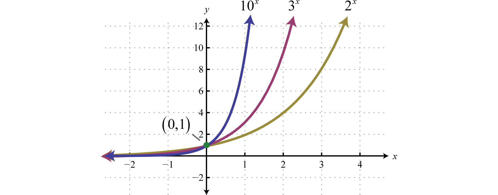
Note that all of these exponential functions have the same \(y\)-intercept, namely \((0, 1)\). This is because \(f (0) = b^{0} = 1\) for any function defined using the form \(f (x) = b^{x}\). As the functions are read from left to right, they are interpreted as increasing or growing exponentially. Furthermore, any exponential function of this form will have a domain that consists of all real numbers \((−∞, ∞)\) and a range that consists of positive values \((0, ∞)\) bounded by a horizontal asymptote at \(y = 0\).
Example \(\PageIndex{1}\):
Sketch the graph and determine the domain and range: \(f(x)=10^{x}+5\).
Solution
The base \(10\) is used often, most notably with scientific notation. Hence, \(10\) is called the common base. In fact, the exponential function \(y = 10^{x}\) is so important that you will find a button \(10^{x}\) dedicated to it on most modern scientific calculators. In this example, we will sketch the basic graph \(y = 10^{x}\) and then shift it up \(5\) units.
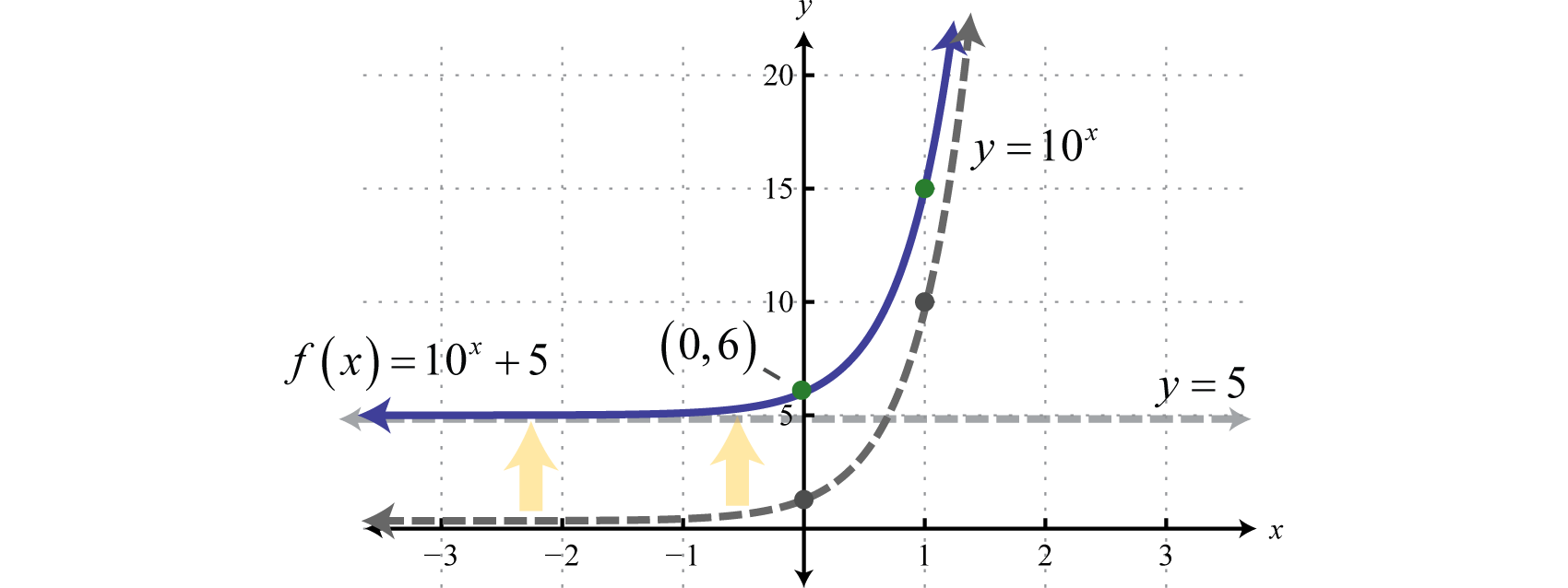
Note that the horizontal asymptote of the basic graph \(y = 10^{x}\) was shifted up \(5\) units to \(y = 5\) (shown dashed). Take a minute to evaluate a few values of \(x\) with your calculator and convince yourself that the result will never be less than \(5\).
Answer
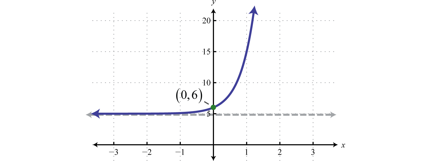
Domain: \((-\infty, \infty)\); Range: \((5, \infty)\)
Next consider exponential functions with fractional bases \(0 < b < 1\). For example, \(f(x)=\left(\frac{1}{2}\right)^{x}\) is an exponential function with base \(b = \frac{1}{2}\).
| \(x\) | \(y\) | \(f(x)=\left(\frac{1}{2}\right)^{x}\) | \(\color{Cerulean}{Solutions} \) |
|---|---|---|---|
| \(-2\) | \(\color{Cerulean}{4} \) | \(f\left(\frac{1}{2}\right)=\left(\frac{1}{2}\right)^{-2}=\frac{1^{-2}}{2^{-2}}=\frac{2^{2}}{1^{2}}=4\) | \((-2,4)\) |
| \(-1\) | \(\color{Cerulean}{2}\) | \(f\left(\frac{1}{2}\right)=\left(\frac{1}{2}\right)^{-1}=\frac{1^{-1}}{2^{-1}}=\frac{2^{1}}{1^{1}}=2\) | \((-1,2)\) |
| \(0\) | \(\color{Cerulean}{1}\) | \(f\left(\frac{1}{2}\right)=\left(\frac{1}{2}\right)^{0}=1\) | \((0,1)\) |
| \(1\) | \(\color{Cerulean}{\frac{1}{2}}\) | \(f\left(\frac{1}{2}\right)=\left(\frac{1}{2}\right)^{1}=\frac{1}{2}\) | \(\left(1, \frac{1}{2}\right)\) |
| \(2\) | \(\color{Cerulean}{\frac{1}{4}}\) | \(f\left(\frac{1}{2}\right)=\left(\frac{1}{2}\right)^{2}=\frac{1}{4}\) | \(\left(2, \frac{1}{4}\right)\) |
Plotting points we have,
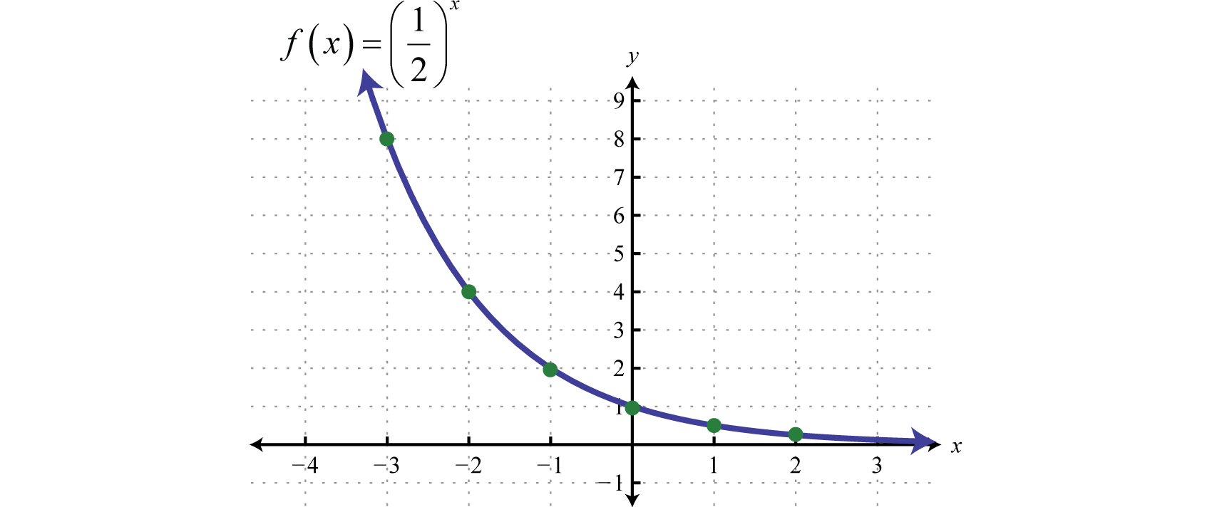
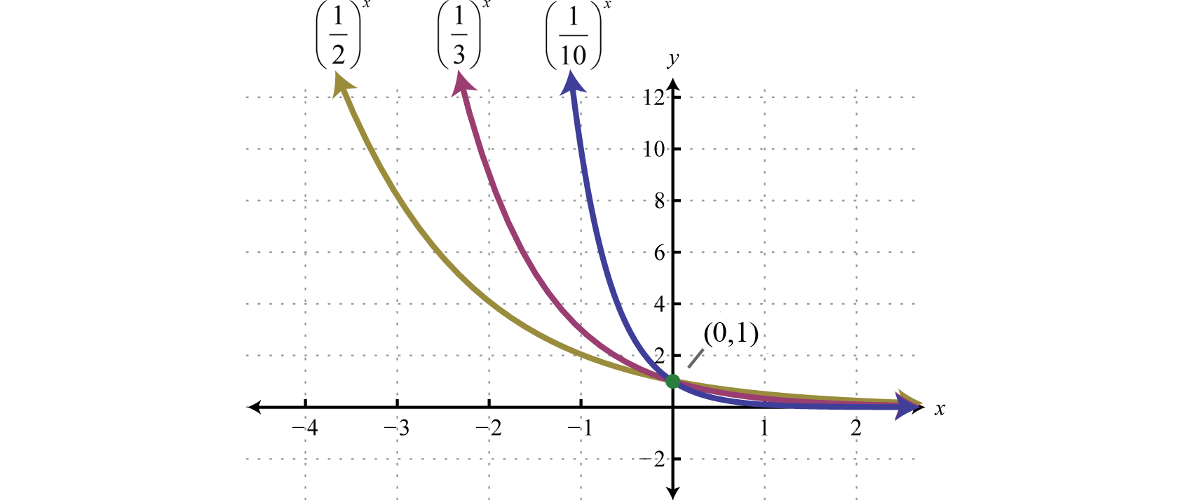
Reading the graph from left to right, it is interpreted as decreasing exponentially. The base affects the rate at which the exponential function decreases or decays. Below we have graphed \(y=\left(\frac{1}{2}\right)^{x}, y=\left(\frac{1}{3}\right)^{x}\), and \(y=\left(\frac{1}{10}\right)^{x}\) on the same set of axes.
Recall that \(x^{-1}=\frac{1}{x}\) and so we can express exponential functions with fractional bases using negative exponents. For example,
\(g(x)=\left(\frac{1}{2}\right)^{x}=\frac{1^{x}}{2^{x}}=\frac{1}{2^{x}}=2^{-x}\)
Furthermore, given that \(f (x) = 2^{x}\) we can see \(g(x)=f(-x)=2^{-x}\) and can consider \(g\) to be a reflection of \(f\) about the \(y\)-axis.

In summary, given \(b > 0\)

And for both cases,
\(\begin{aligned}\color{Cerulean} { Domain :}&(-\infty, \infty) \\ \color{Cerulean} { Range : }&(0, \infty) \\ \color{Cerulean} { y-intercept : }&(0,1) \\ \color{Cerulean} { Asymptote: }& y=0\end{aligned}\)
Furthermore, note that the graphs pass the horizontal line test and thus exponential functions are one-to-one. We use these basic graphs, along with the transformations, to sketch the graphs of exponential functions.
Example \(\PageIndex{2}\)
Sketch the graph and determine the domain and range: \(f(x)=5^{-x}-10\).
Solution
Begin with the basic graph \(y = 5^{−x}\) and shift it down \(10\) units.
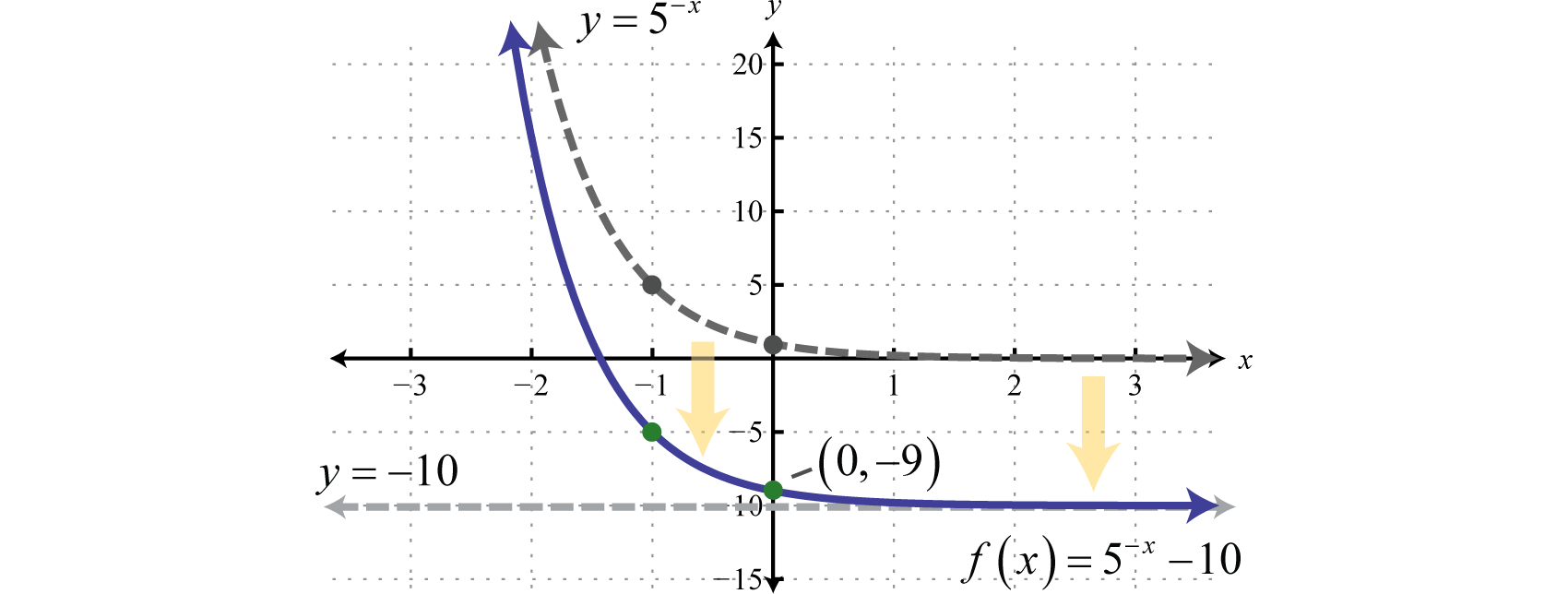
The \(y\)-intercept is \((0, −9)\) and the horizontal asymptote is \(y = −10\).
Answer
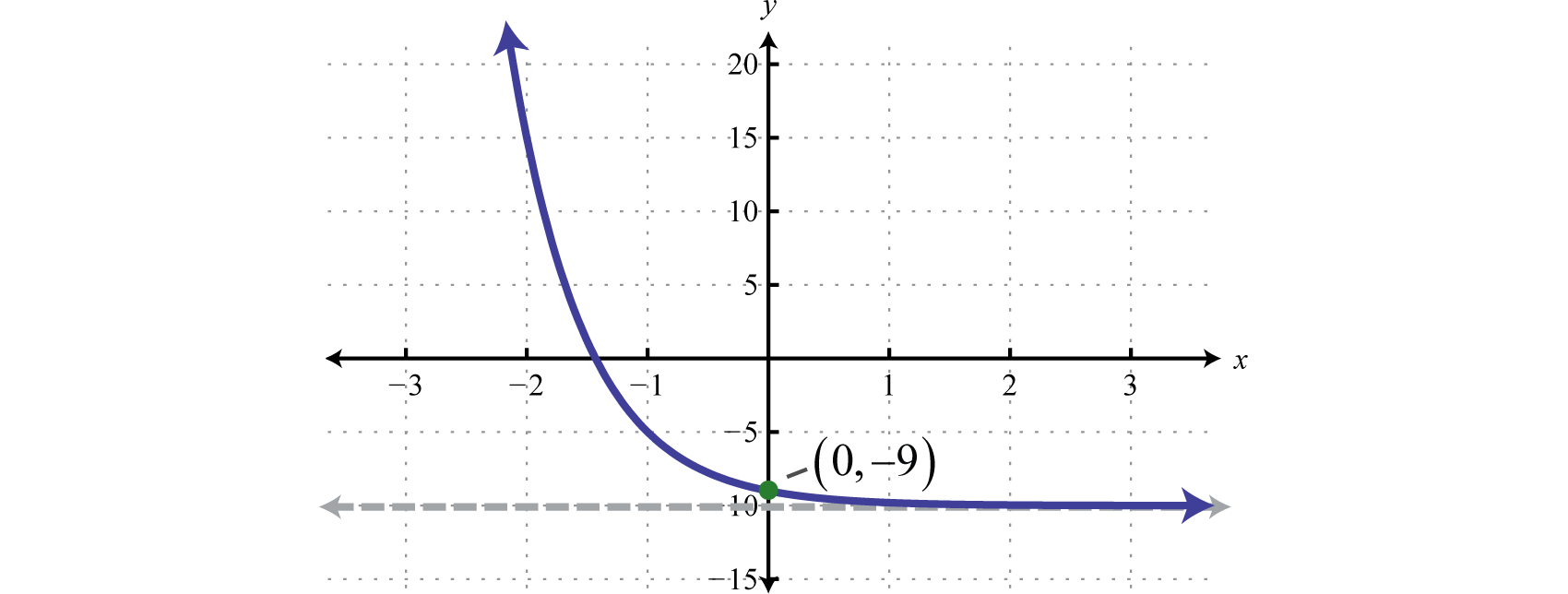
Domain: \((-\infty, \infty)\); Range: \((-10, \infty)\)
Finding the \(x\)-intercept of the graph in the previous example is left for a later section in this chapter. For now, we are more concerned with the general shape of exponential functions.
Example \(\PageIndex{3}\)
Sketch the graph and determine the domain and range of \(g(x)=-2^{x-3}\).
Solution
Begin with the basic graph \(y=2^{x}\) and identify the transformations.
\(\begin{array}{l}{y=2^{x}} \quad\quad\quad\color{Cerulean}{Basic\:graph} \\ {y=-2^{x}} \quad\:\:\:\:\color{Cerulean}{Reflection\:about\:the\:x-axis} \\ {y=-2^{x-3}}\quad\color{Cerulean}{Shift\:right\:3\:units}\end{array}\)
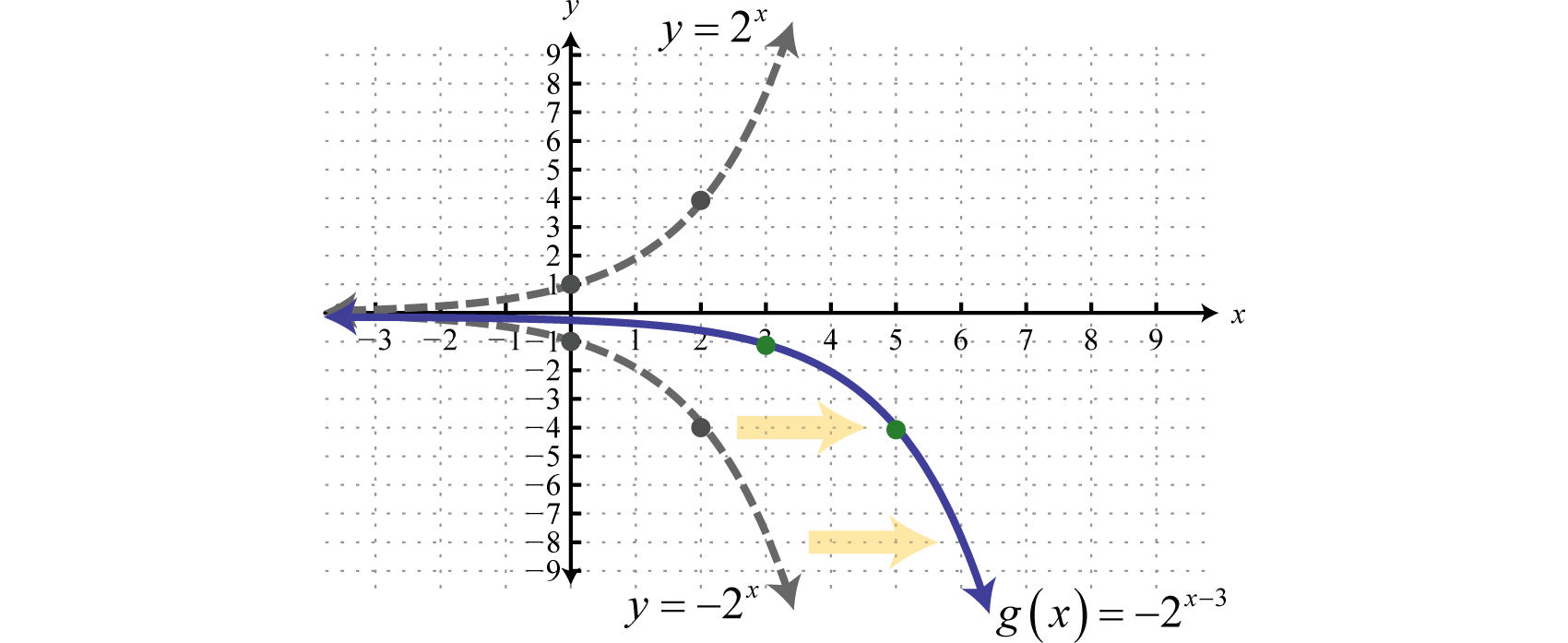
Note that the horizontal asymptote remains the same for all of the transformations. To finish we usually want to include the \(y\)-intercept. Remember that to find the \(y\)-intercept we set \(x = 0\).
\(\begin{aligned} g(\color{Cerulean}{0}\color{black}{)} &=-2^{\color{Cerulean}{0}\color{black}{-}3} \\ &=-2^{-3} \\ &=-\frac{1}{2^{3}} \\ &=-\frac{1}{8} \end{aligned}\)
Therefore the \(y\)-intercept is \(\left(0,-\frac{1}{8}\right)\).
Answer
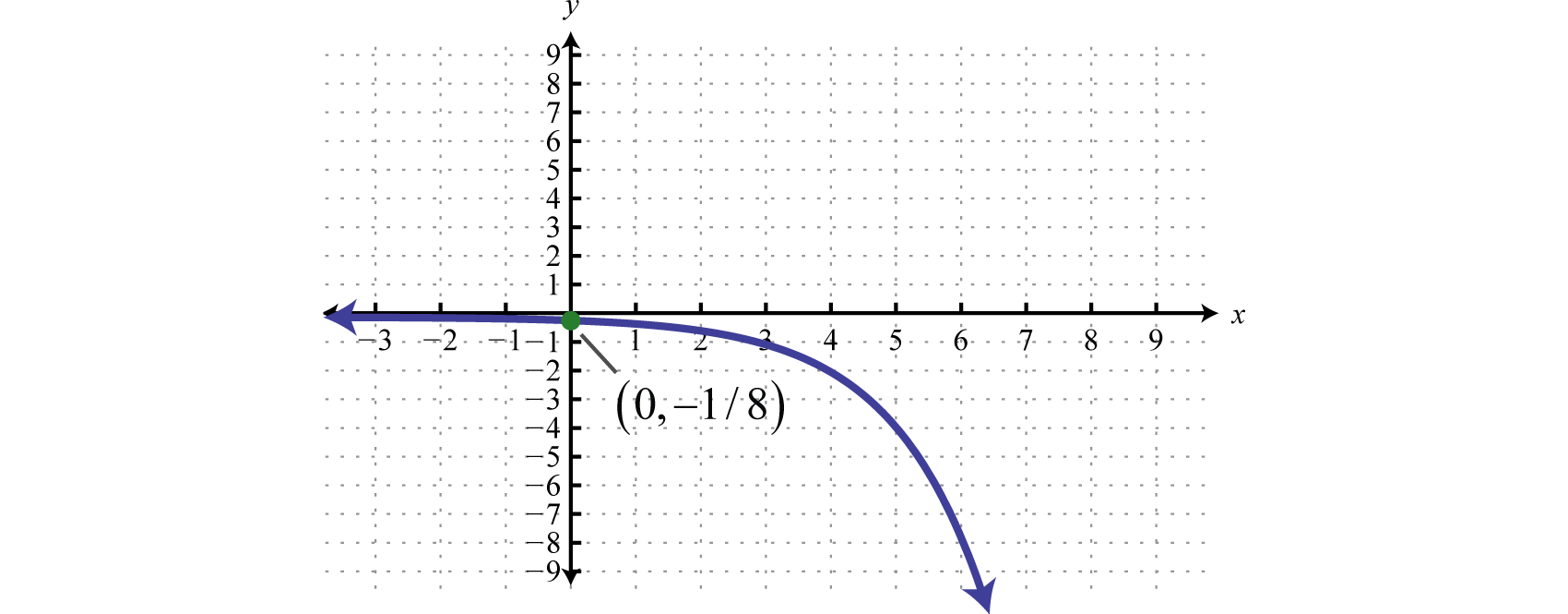
Domain: \((-\infty, \infty)\); Range: \((-\infty, 0)\)
Exercise \(\PageIndex{1}\)
Sketch the graph and determine the domain and range: \(f(x)=2^{x-1}+3\)
- Answer
-
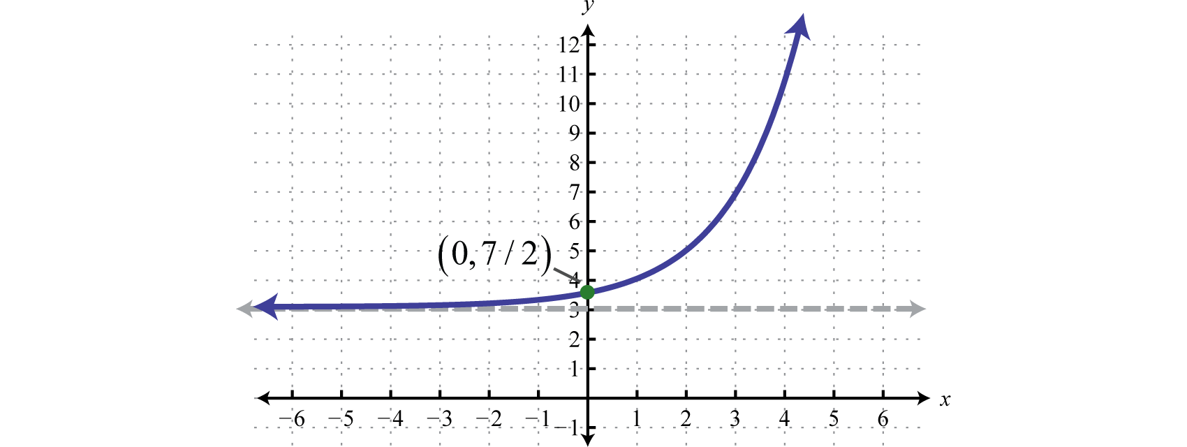
Figure \(\PageIndex{13}\) Domain: \((-\infty, \infty)\); Range: \((3, \infty)\)
www.youtube.com/v/WDcObqDtE7M
Natural Base e
Some numbers occur often in common applications. One such familiar number is pi (\(π\)), which we know occurs when working with circles. This irrational number has a dedicated button on most calculators \(π\) and approximated to five decimal places, \(π ≈ 3.14159\). Another important number \(e\) occurs when working with exponential growth and decay models. It is an irrational number and approximated to five decimal places, \(e ≈ 2.71828\). This constant occurs naturally in many real-world applications and thus is called the natural base. Sometimes \(e\) is called Euler’s constant in honor of Leonhard Euler (pronounced “Oiler”).

Figure \(\PageIndex{14}\): Leonhard Euler (1707-1783)
In fact, the natural exponential funnction:
\(f(x)=e^{x}\)
is so important that you will find a button \(e^{x}\) dedicated to it on any modern scientific calculator. In this section, we are interested in evaluating the natural exponential function for given real numbers and sketching its graph. To evaluate the natural exponential function, defined by \(f (x) = e^{x}\) where \(x = −2\) using a calculator, you may need to apply the shift button. On many scientific calculators the caret will display as follows,
\(f(-2)=e^{\wedge}(-2) \approx 0.13534\)
After learning how to use your particular calculator, you can now sketch the graph by plotting points. (Round off to the nearest hundredth.)
| \(x\) | \(y\) | \(f(x)=e^{x}\) | \(\color{Cerulean}{Solutions} \) |
|---|---|---|---|
| \(-2\) | \(\color{Cerulean}{0.14}\) | \(f(-2)=e^{-2}=0.14\) | \((-2,0.14)\) |
| \(-1\) | \(\color{Cerulean}{0.37}\) | \(f(-1)=e^{-1}=0.37\) | \((-1,0.37)\) |
| \(0\) | \(\color{Cerulean}{1}\) | \(f(0)=e^{0}=1\) | \((0,1)\) |
| \(1\) | \(\color{Cerulean}{2.72}\) | \(f(1)=e^{1}=2.72\) | \((1,2.72)\) |
| \(2\) | \(\color{Cerulean}{7.39}\) | \(f(2)=e^{2}=7.39\) | \((2,7.39)\) |
Plot the points and sketch the graph.
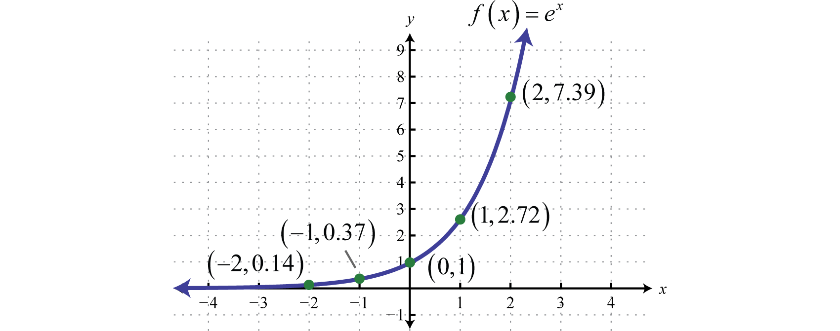
Note that the function is similar to the graph of \(y = 3^{x}\). The domain consists of all real numbers and the range consists of all positive real numbers. There is an asymptote at \(y = 0\) and a \(y\)-intercept at \((0, 1)\). We can use the transformations to sketch the graph of more complicated exponential functions.
Example \(\PageIndex{4}\):
Sketch the graph and determine the domain and range: \(g(x)=e^{x+2}-3\).
Solution
Identify the basic transformations.
\(\begin{array}{l}{y=e^{x}} \quad\quad\quad\:\:\:\color{Cerulean}{Basic\:graph} \\ {y=e^{x+2}} \quad\quad\:\:\:\color{Cerulean}{Shift\:left\:2\:units}\\ {y=e^{x+2}-3}\:\:\:\:\color{Cerulean}{Shift\:down\:3\:units}\end{array}\)
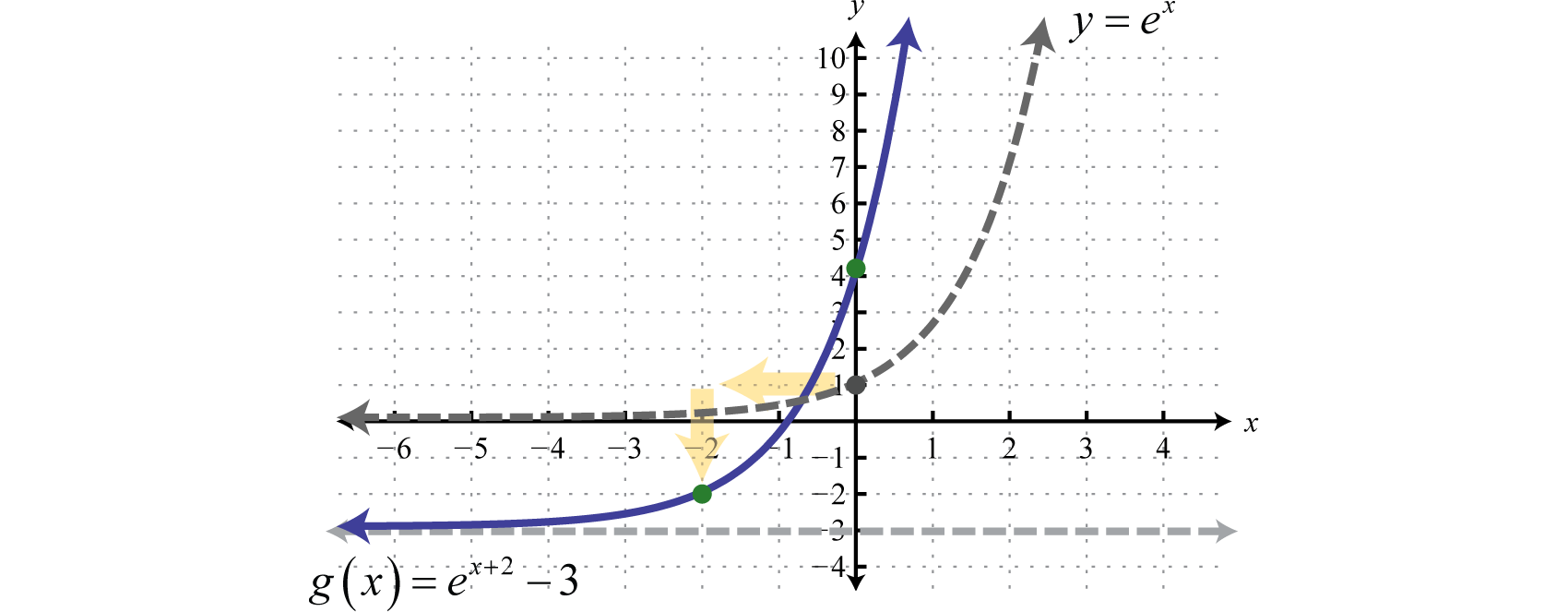
To determine the \(y\)-intercept set \(x = 0\).
\(\begin{aligned} g(\color{Cerulean}{0}\color{black}{)} &=e^{\color{Cerulean}{0}\color{black}{+}2}-3 \\ &=e^{2}-3 \\ & \approx 4.39 \end{aligned}\)
Therefore the \(y\)-intercept is \((0, e^{2} − 3)\).
Answer
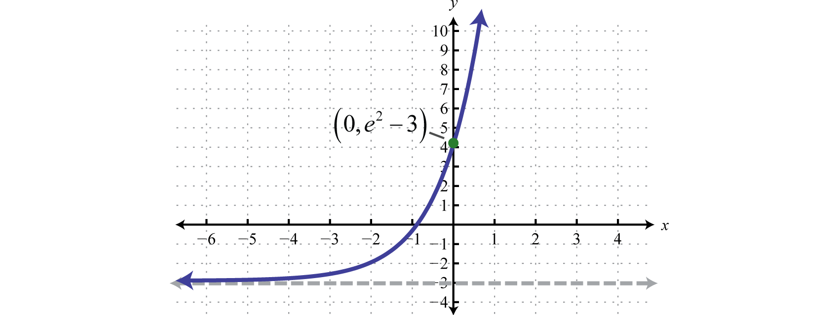
Domain: \((-\infty, \infty)\); Range: \((-3, \infty)\)
Exercise \(\PageIndex{2}\)
Sketch the graph and determine the domain and range: \(f(x)=e^{-x}+2\).
- Answer
-
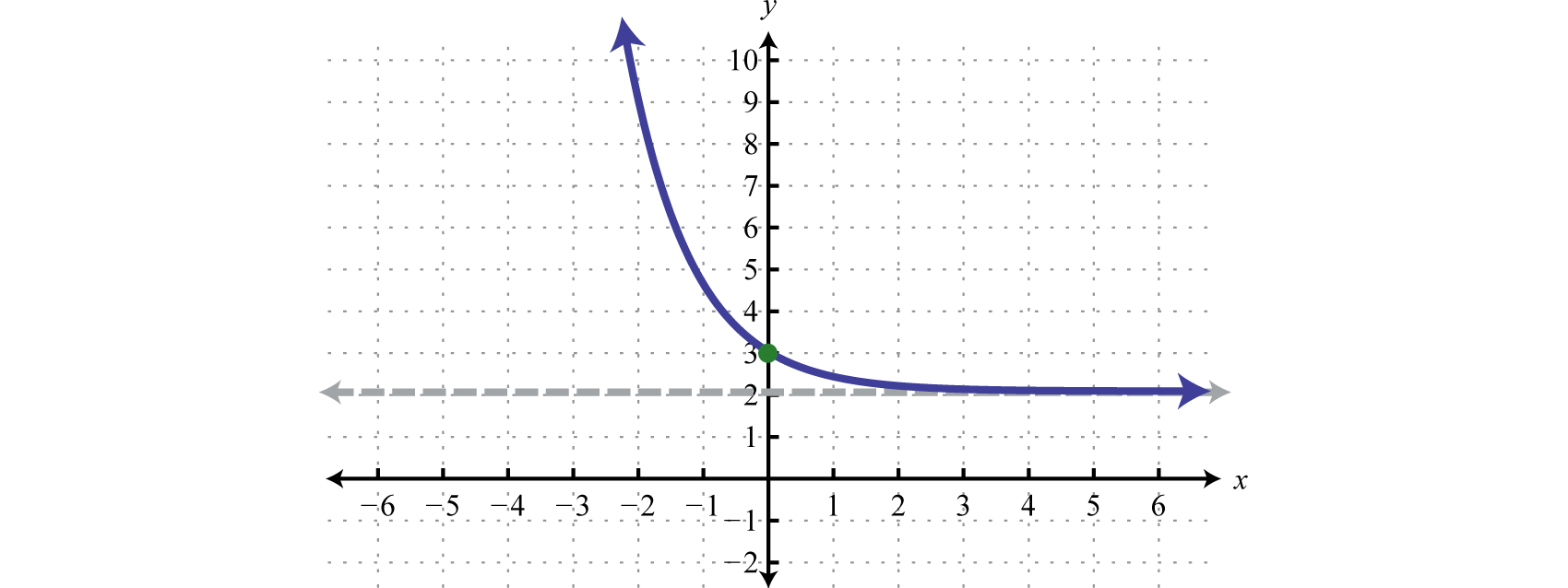
Figure \(\PageIndex{18}\) Domain: \((-\infty, \infty)\); Range: \((2, \infty)\)
www.youtube.com/v/FkwBpg2Xpb8
Compound Interest Formulas
Exponential functions appear in formulas used to calculate interest earned in most regular savings accounts. Compound interest occurs when interest accumulated for one period is added to the principal investment before calculating interest for the next period. The amount accrued in this manner over time is modeled by the compound interest formula6:
\(A(t)=P\left(1+\frac{r}{n}\right)^{n t}\)
Here the amount \(A\) depends on the time \(t\) in years the principal \(P\) is accumulating compound interest at an annual interest rate \(r\). The value \(n\) represents the number of times the interest is compounded in a year.
Example \(\PageIndex{5}\):
An investment of $\(500\) is made in a \(6\)-year CD that earns \(4 \frac{1}{2}\)% annual interest that is compounded monthly. How much will the CD be worth at the end of the \(6\)-year term?
Solution
Here the principal \(P =\) $\(500\), the interest rate \(r = 4 \frac{1}{2}\)% \(= 0.045\), and because the interest is compounded monthly, \(n = 12\). The investment is modeled by the following,
\(A(t)=500\left(1+\frac{0.045}{12}\right)^{12 t}\)
To determine the amount in the account after \(6\) years evaluate \(A (6)\) and round off to the nearest cent.
\(\begin{aligned} A(\color{Cerulean}{6}\color{black}{)} &=500\left(1+\frac{0.045}{12}\right)^{12(\color{Cerulean}{6}\color{black}{)}} \\ &=500(1.00375)^{72} \\ &=654.65 \end{aligned}\)
Answer
The CD will be worth $\(654.65\) at the end of the \(6\)-year term.
Next we explore the effects of increasing \(n\) in the formula. For the sake of clarity we let \(P\) and \(r\) equal \(1\) and calculate accordingly.
| Annual Compounding | \(\left(1+\frac{1}{n}\right)^{n}\) |
|---|---|
| Yearly \((n=1)\) | \(\color{black}{\left(1+\frac{1}{\color{Cerulean}{1}}\right)}^{\color{Cerulean}{1}}\color{black}{=}2\) |
| Semi-annually \((n=2)\) | \(\color{black}{\left(1+\frac{1}{\color{Cerulean}{2}}\right)}^{\color{Cerulean}{2}}\color{black}{=}2.25\) |
| Quarterly \((n=4)\) | \(\color{black}{\left(1+\frac{1}{\color{Cerulean}{4}}\right)}^{\color{Cerulean}{4}}\color{black}{≈}2.44140\) |
| Monthly \((n=12)\) | \(\color{black}{\left(1+\frac{1}{\color{Cerulean}{12}}\right)}^{\color{Cerulean}{12}}\color{black}{≈}2.61304\) |
| Weekly \((n=52)\) | \(\color{black}{\left(1+\frac{1}{\color{Cerulean}{52}}\right)}^{\color{Cerulean}{52}}\color{black}{≈}2.69260\) |
| Daily \((n=365)\) | \(\color{black}{\left(1+\frac{1}{\color{Cerulean}{365}}\right)}^{\color{Cerulean}{365}}\color{black}{≈}2.71457\) |
| Hourly \((n=8760)\) | \(\color{black}{\left(1+\frac{1}{\color{Cerulean}{8760}}\right)}^{\color{Cerulean}{8760}}\color{black}{≈}2.71813\) |
Continuing this pattern, as \(n\) increases to say compounding every minute or even every second, we can see that the result tends toward the natural base \(e ≈ 2.71828\). Compounding interest every instant leads to the continuously compounding interest formula7,
\(A(t)=P e^{rt}\)
Here \(P\) represents the initial principal amount invested, \(r\) represents the annual interest rate, and \(t\) represents the time in years the investment is allowed to accrue continuously compounded interest.
Example \(\PageIndex{6}\):
An investment of $\(500\) is made in a \(6\)-year CD that earns \(4 \frac{1}{2}\)% annual interest that is compounded continuously. How much will the CD be worth at the end of the \(6\)-year term?
Solution
Here the principal \(P =\) $\(500\), and the interest rate \(r = 4 \frac{1}{2}\)% \(= 0.045\). Since the interest is compounded continuously we will use the formula \(A (t) = Pe^{rt}\). The investment is modeled by the following,
\(A(t)=500 e^{0.045 t}\)
To determine the amount in the account after \(6\) years, evaluate \(A (6)\) and round off to the nearest cent.
\(\begin{aligned} A(\color{Cerulean}{6}\color{black}{)} &=500 e^{0.045(\color{Cerulean}{6}\color{black}{)}} \\ &=500 e^{0.27} \\ &=654.98 \end{aligned}\)
Answer
The CD will be worth $\(654.98\) at the end of the \(6\)-year term.
Compare the previous two examples and note that compounding continuously may not be as beneficial as it sounds. While it is better to compound interest more often, the difference is not that profound. Certainly, the interest rate is a much greater factor in the end result.
Exercise \(\PageIndex{3}\)
How much will a $\(1,200\) CD, earning \(5.2\)% annual interest compounded continuously, be worth at the end of a \(10\)-year term?
- Answer
-
$\(2,018.43\)
www.youtube.com/v/1alUOjTq5wc
Key Takeaways
- Exponential functions have definitions of the form \(f (x) = b^{x}\) where \(b > 0\) and \(b ≠ 1\). The domain consists of all real numbers \((−∞, ∞)\) and the range consists of positive numbers \((0, ∞)\). Also, all exponential functions of this form have a \(y\)-intercept of \((0, 1)\) and are asymptotic to the \(x\)-axis.
- If the base of an exponential function is greater than \(1 (b > 1)\), then its graph increases or grows as it is read from left to right.
- If the base of an exponential function is a proper fraction \((0 < b < 1)\), then its graph decreases or decays as it is read from left to right.
- The number \(10\) is called the common base and the number \(e\) is called the natural base.
- The natural exponential function defined by \(f (x) = e^{x}\) has a graph that is very similar to the graph of \(g (x) = 3^{x}\).
- Exponential functions are one-to-one.
Exercise \(\PageIndex{4}\)
Evaluate.
- \(f(x)=3^{x}\) where \(f(-2), f(0),\) and \(f(2)\).
- \(f(x)=10^{x}\) where \(f(-1), f(0),\) and \(f(1)\).
- \(g(x)=\left(\frac{1}{3}\right)^{x}\) where \(g(-1), g(0),\) and \(g(3)\).
- \(g(x)=\left(\frac{3}{4}\right)^{x}\) where \(g(-2), g(-1),\) and \(g(0)\).
- \(h(x)=9^{-x}\) where \(h(-1), h(0),\) and \(h\left(\frac{1}{2}\right)\).
- \(h(x)=4^{-x}\) where \(h(-1), h\left(-\frac{1}{2}\right),\) and \(h(0)\).
- \(f(x)=-2^{x}+1\) where \(f(-1), f(0),\) and \(f(3)\).
- \(f(x)=2-3^{x}\) where \(f(-1), f(0),\) and \(f(2)\).
- \(g(x)=10^{-x}+20\) where \(g(-2), g(-1),\) and \(g(0)\).
- \(g(x)=1-2^{-x}\) where \(g(-1), g(0),\) and \(g(1)\).
- Answer
-
1. \(f(-2)=\frac{1}{9}, f(0)=1, f(2)=9\)
3. \(g(-1)=3, g(0)=1, g(3)=\frac{1}{27}\)
5. \(h(-1)=9, h(0)=1, h\left(\frac{1}{2}\right)=\frac{1}{3}\)
7. \(f(-1)=\frac{1}{2}, f(0)=0, f(3)=-7\)
9. \(g(-2)=120, g(-1)=30, g(0)=21\)
Exercise \(\PageIndex{5}\)
Use a calculator to approximate the following to the nearest hundredth.
- \(f(x)=2^{x}+5\) where \(f(2.5)\).
- \(f(x)=3^{x}-10\) where \(f(3.2)\).
- \(g(x)=4^{x}\) where \(g(\sqrt{2})\).
- \(g(x)=5^{x}-1\) where \(g(\sqrt{3})\).
- \(h(x)=10^{x}\) where \(h(\pi)\).
- \(h(x)=10^{x} + 1\) where \(h\left(\frac{\pi}{3}\right)\).
- \(f(x)=10^{-x}-2\) where \(f(1.5)\).
- \(f(x)=5^{-x}+3\) where \(f(1.3)\).
- \(f(x)=\left(\frac{2}{3}\right)^{x}+1\) where \(f(-2.7)\).
- \(f(x)=\left(\frac{3}{5}\right)^{-x}-1\) where \(f(1.4)\).
- Answer
-
1. \(10.66\)
3. \(7.10\)
5. \(1385.46\)
7. \(−1.97\)
9. \(3.99\)
Exercise \(\PageIndex{6}\)
Sketch the function and determine the domain and range. Draw the horizontal asymptote with a dashed line.
- \(f(x)=4^{x}\)
- \(g(x)=3^{x}\)
- \(f(x)=4^{x}+2\)
- \(f(x)=3^{x}-6\)
- \(f(x)=2^{x-2}\)
- \(f(x)=4^{x+2}\)
- \(f(x)=3^{x+1}-4\)
- \(f(x)=10^{x-4}+2\)
- \(h(x)=2^{x-3}-2\)
- \(h(x)=3^{x+2}+4\)
- \(f(x)=\left(\frac{1}{4}\right)^{x}\)
- \(h(x)=\left(\frac{1}{3}\right)^{x}\)
- \(f(x)=\left(\frac{1}{4}\right)^{x}-2\)
- \(h(x)=\left(\frac{1}{3}\right)^{x}+2\)
- \(g(x)=2^{-x}-3\)
- \(g(x)=3^{-x}+1\)
- \(f(x)=6-10^{-x}\)
- \(g(x)=5-4^{-x}\)
- \(f(x)=5-2^{x}\)
- \(f(x)=3-3^{x}\)
- Answer
-
1. Domain: \((-\infty, \infty)\); Range: \((0, \infty)\)
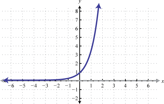
Figure \(\PageIndex{19}\) 3. Domain: \((-\infty, \infty)\); Range: \((2, \infty)\)
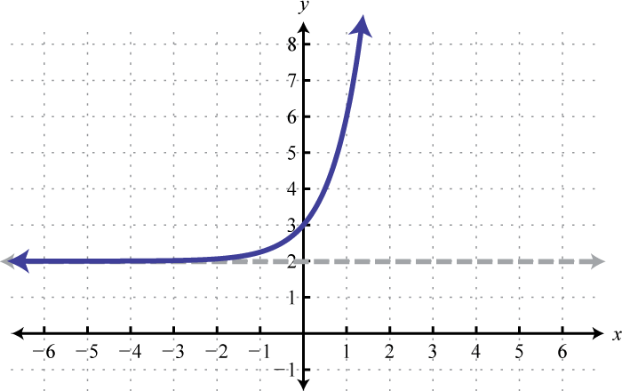
Figure \(\PageIndex{20}\) 5. Domain: \((-\infty, \infty)\); Range: \((0, \infty)\)
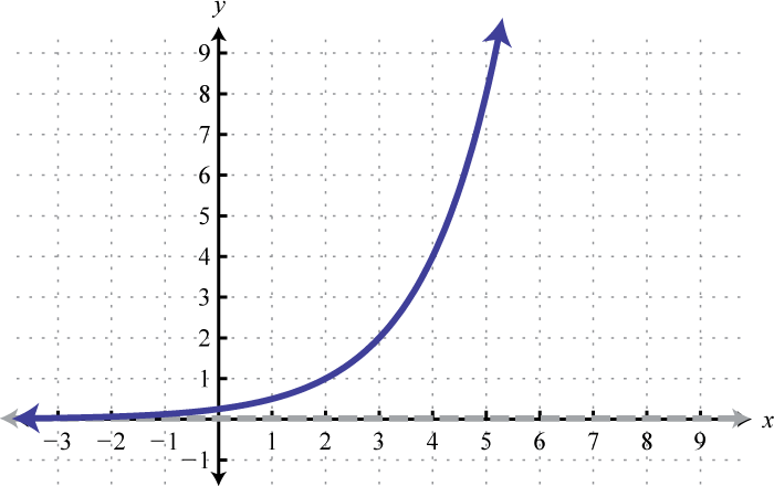
Figure \(\PageIndex{21}\) 7. Domain: \((-\infty, \infty)\); Range: \((-4, \infty)\)
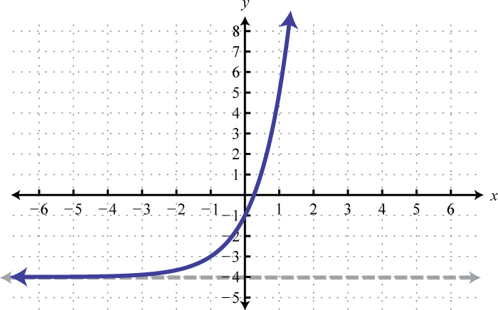
Figure \(\PageIndex{22}\) 9. Domain: \((-\infty, \infty)\); Range: \((-2, \infty)\)
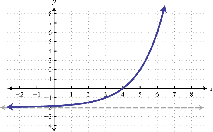
Figure \(\PageIndex{23}\) 11. Domain: \((-\infty, \infty)\); Range: \((0, \infty)\)
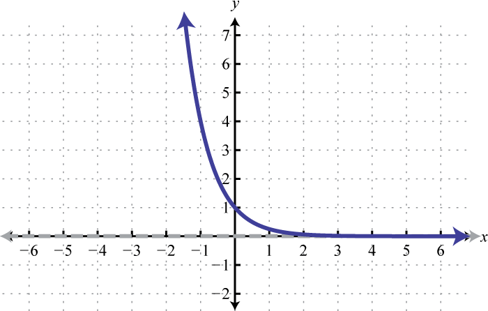
Figure \(\PageIndex{24}\) 13. Domain: \((-\infty, \infty)\); Range: \((-2, \infty)\)
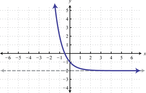
Figure \(\PageIndex{25}\) 15. Domain: \((-\infty, \infty)\); Range: \((-3, \infty)\)
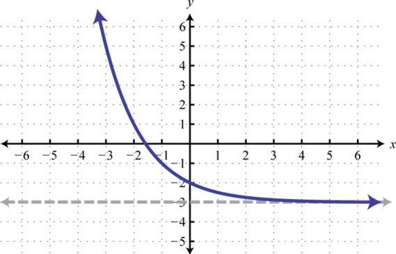
Figure \(\PageIndex{26}\) 17. Domain: \((-\infty, \infty)\); Range: \((-\infty, 6)\)

Figure \(\PageIndex{27}\) 19. Domain: \((-\infty, \infty)\); Range: \((-\infty, 5)\)
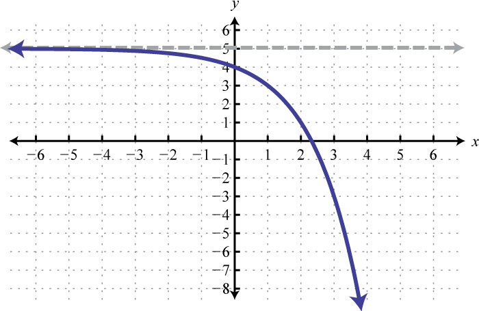
Figure \(\PageIndex{28}\)
Exercise \(\PageIndex{7}\)
Find \(f (−1), f (0)\), and \(f (\frac{3}{2})\) for the given function. Use a calculator where appropriate to approximate to the nearest hundredth.
- \(f(x)=e^{x}+2\)
- \(f(x)=e^{x}-4\)
- \(f(x)=5-3 e^{x}\)
- \(f(x)=e^{-x}+3\)
- \(f(x)=1+e^{-x}\)
- \(f(x)=3-2 e^{-x}\)
- \(f(x)=e^{-2 x}+2\)
- \(f(x)=e^{-x^{2}}-1\)
- Answer
-
1. \(f(-1) \approx 2.37, f(0)=3, f\left(\frac{3}{2}\right) \approx 6.48\)
3. \(f(-1) \approx 3.90, f(0)=2, f\left(\frac{3}{2}\right) \approx-8.45\)
5. \(f(-1) \approx 3.72, f(0)=2, f\left(\frac{3}{2}\right) \approx 1.22\)
7. \(f(-1) \approx 9.39, f(0)=3, f\left(\frac{3}{2}\right) \approx 2.05\)
Exercise \(\PageIndex{8}\)
Sketch the function and determine the domain and range. Draw the horizontal asymptote with a dashed line.
- \(f(x)=e^{x}-3\)
- \(f(x)=e^{x}+2\)
- \(f(x)=e^{x+1}\)
- \(f(x)=e^{x-3}\)
- \(f(x)=e^{x-2}+1\)
- \(f(x)=e^{x+2}-1\)
- \(g(x)=-e^{x}\)
- \(g(x)=e^{-x}\)
- \(h(x)=-e^{x+1}\)
- \(h(x)=-e^{x}+3\)
- Answer
-
1. Domain: \((-\infty, \infty)\); Range: \((-3, \infty)\)
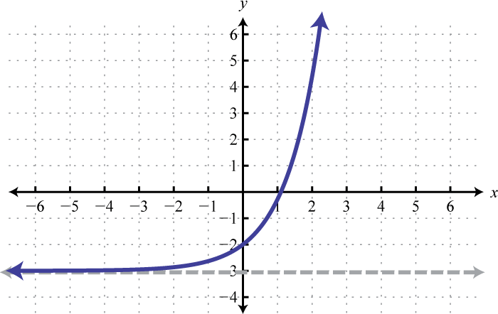
Figure \(\PageIndex{29}\) 3. Domain: \((-\infty, \infty)\); Range: \((0, \infty)\)
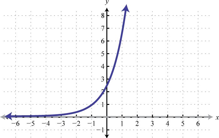
Figure \(\PageIndex{30}\) 5. Domain: \((-\infty, \infty)\); Range: \((1, \infty)\)
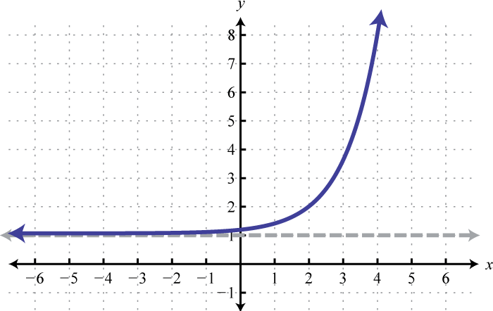
Figure \(\PageIndex{31}\) 7. Domain: \((-\infty, \infty)\); Range: \((-\infty, 0)\)
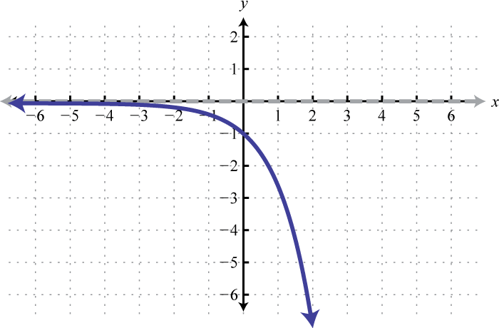
Figure \(\PageIndex{32}\) 9. Domain: \((-\infty, \infty)\); Range: \((-\infty, 0)\)
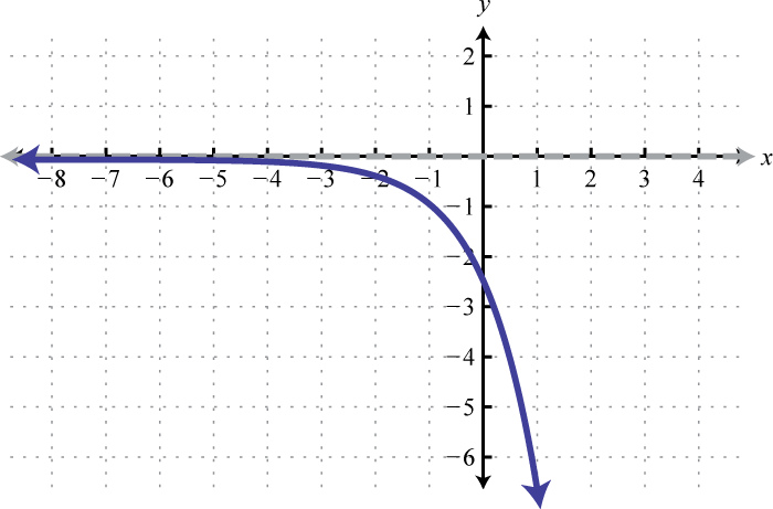
Figure \(\PageIndex{33}\)
Exercise \(\PageIndex{9}\)
- Jim invested $\(750\) in a \(3\)-year CD that earns \(4.2\)% annual interest that is compounded monthly. How much will the CD be worth at the end of the \(3\)-year term?
- Jose invested $\(2,450\) in a \(4\)-year CD that earns \(3.6\)% annual interest that is compounded semi-annually. How much will the CD be worth at the end of the \(4\)-year term?
- Jane has her $\(5,350\) savings in an account earning \(3 \frac{5}{8}\)% annual interest that is compounded quarterly. How much will be in the account at the end of \(5\) years?
- Bill has $\(12,400\) in a regular savings account earning \(4 \frac{2}{3}\)% annual interest that is compounded monthly. How much will be in the account at the end of \(3\) years?
- If $\(85,200\) is invested in an account earning \(5.8\)% annual interest compounded quarterly, then how much interest is accrued in the first \(3\) years?
- If $\(124,000\) is invested in an account earning \(4.6\)% annual interest compounded monthly, then how much interest is accrued in the first \(2\) years?
- Bill invested $\(1,400\) in a \(3\)-year CD that earns \(4.2\)% annual interest that is compounded continuously. How much will the CD be worth at the end of the \(3\)-year term?
- Brooklyn invested $\(2,850\) in a \(5\)-year CD that earns \(5.3\)% annual interest that is compounded continuously. How much will the CD be worth at the end of the \(5\)-year term?
- Omar has his $\(4,200\) savings in an account earning \(4 \frac{3}{8}\)% annual interest that is compounded continuously. How much will be in the account at the end of \(2 \frac{1}{2}\) years?
- Nancy has her $\(8,325\) savings in an account earning \(5 \frac{7}{8}\)% annual interest that is compounded continuously. How much will be in the account at the end of \(5 \frac{1}{2}\) years?
- If $\(12,500\) is invested in an account earning \(3.8\)% annual interest compounded continuously, then how much interest is accrued in the first \(10\) years?
- If $\(220,000\) is invested in an account earning \(4.5\)% annual interest compounded continuously, then how much interest is accrued in the first \(2\) years?
- The population of a certain small town is growing according to the function \(P (t) = 12,500(1.02)^{t}\) where \(t\) represents time in years since the last census. Use the function to determine the population on the day of the census (when \(t = 0\)) and estimate the population in \(6\) years from that time.
- The population of a certain small town is decreasing according to the function \(P (t) = 22,300(0.982)^{t}\) where \(t\) represents time in years since the last census. Use the function to determine the population on the day of the census (when \(t = 0\)) and estimate the population in \(6\) years from that time.
- The decreasing value, in dollars, of a new car is modeled by the formula \(V (t) = 28,000(0.84)^{t}\) where \(t\) represents the number of years after the car was purchased. Use the formula to determine the value of the car when it was new (\(t = 0\)) and the value after \(4\) years.
- The number of unique visitors to the college website can be approximated by the formula \(N (t) = 410(1.32)^{t}\) where \(t\) represents the number of years after 1997 when the website was created. Approximate the number of unique visitors to the college website in the year 2020.
- If left unchecked, a new strain of flu virus can spread from a single person to others very quickly. The number of people affected can be modeled using the formula \(P(t)=e^{0.22 t}\) where \(t\) represents the number of days the virus is allowed to spread unchecked. Estimate the number of people infected with the virus after \(30\) days and after \(60\) days.
- If left unchecked, a population of \(24\) wild English rabbits can grow according to the formula \(P(t)=24 e^{0.19 t}\) where the time \(t\) is measured in months. How many rabbits would be present \(3 \frac{1}{2}\) years later?
- The population of a certain city in 1975 was \(65,000\) people and was growing exponentially at an annual rate of \(1.7\)%. At the time, the population growth was modeled by the formula \(P (t) = 65,000e^{0.017t}\) where \(t\) represented the number of years since 1975. In the year 2000, the census determined that the actual population was \(104,250\) people. What population did the model predict for the year 2000 and what was the actual error?
- Because of radioactive decay, the amount of a \(10\) milligram sample of Iodine-131 decreases according to the formula \(A (t) = 10e^{−0.087t}\) where \(t\) represents time measured in days. How much of the sample remains after \(10\) days?
- The number of cells in a bacteria sample is approximated by the logistic growth model \(N(t)=\frac{1.2 \times 10^{5}}{1+9 e^{-0.32 t}}\) where \(t\) represents time in hours. Determine the initial number of cells and then determine the number of cells \(6\) hours later.
- The market share of a product, as a percentage, is approximated by the formula \(P(t)=\frac{100}{2+e^{-0.44 t}}\) where \(t\) represents the number of months after an aggressive advertising campaign is launched. By how much can we expect the market share to increase after the first three months of advertising?
- Answer
-
1. $\(850.52\)
3. $\(6,407.89\)
5. $\(16,066.13\)
7. $\(1,588.00\)
9. $\(4,685.44\)
11. $\(5,778.56\)
13. Initial population: \(12,500\); Population \(6\) years later: \(14,077\)
15. New: $\(28,000\); In \(4\) years: $\(13,940.40\)
17. After \(30\) days: \(735\) people; After \(60\) days: \(540,365\) people
19. Model: \(99,423\) people; error: \(4,827\) people
21. Initially there are \(12,000\) cells and \(6\) hours later there are \(51,736\) cells.
Exercise \(\PageIndex{10}\)
- Why is \(b = 1\) excluded as a base in the definition of exponential functions? Explain.
- Explain why an exponential function of the form \(y = b^{x}\) can never be negative.
- Research and discuss the derivation of the compound interest formula.
- Research and discuss the logistic growth model. Provide a link to more information on this topic.
- Research and discuss the life and contributions of Leonhard Euler.
- Answer
-
1. Answer may vary
3. Answer may vary
5. Answer may vary
Footnotes
5Any function with a definition of the form \(f (x) = b^{x}\) where \(b > 0\) and \(b ≠ 1\).
6A formula that gives the amount accumulated by earning interest on principal and interest over time: \(A(t)=P\left(1+\frac{r}{n}\right)^{n t}\).
7A formula that gives the , amount accumulated by earning continuously compounded interest: \(A (t) = Pe^{rt}\).