
2.4: Graphing the Basic Functions
- Page ID
- 6236
Learning Objectives
- Define and graph seven basic functions.
- Define and graph piecewise functions.
- Evaluate piecewise defined functions.
- Define the greatest integer function.
Basic Functions
In this section we graph seven basic functions that will be used throughout this course. Each function is graphed by plotting points. Remember that \(f (x) = y\) and thus \(f (x)\) and \(y\) can be used interchangeably.
Any function of the form \(f (x) = c\), where \(c\) is any real number, is called a constant function43. Constant functions are linear and can be written \(f (x) = 0x + c\). In this form, it is clear that the slope is \(0\) and the \(y\)-intercept is \((0, c)\). Evaluating any value for \(x\), such as \(x = 2\), will result in \(c\).
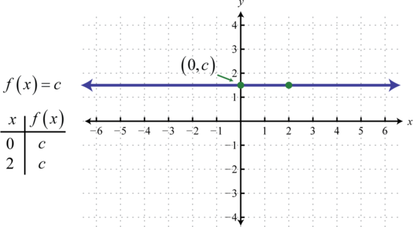
The graph of a constant function is a horizontal line. The domain consists of all real numbers \(ℝ\) and the range consists of the single value \(\{c\}\).
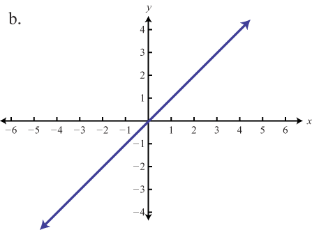
We next define the identity function44 \(f (x) = x\). Evaluating any value for \(x\) will result in that same value. For example, \(f (0) = 0\) and \(f (2) = 2\). The identity function is linear, \(f (x) = 1x + 0\), with slope \(m = 1\) and \(y\)-intercept \((0, 0)\).
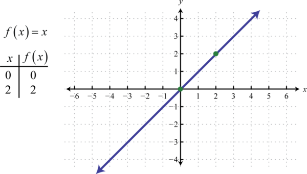
The domain and range both consist of all real numbers.
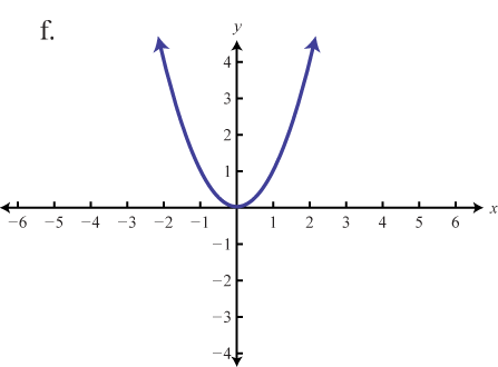
The squaring function45, defined by \(f (x) = x^{2}\), is the function obtained by squaring the values in the domain. For example, \(f (2) = (2)^{2} = 4\) and \(f (−2) = (−2)^{2} = 4\).The result of squaring nonzero values in the domain will always be positive.
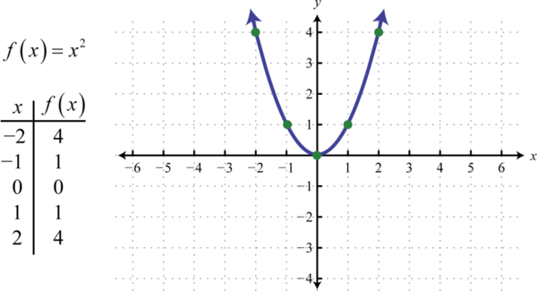
The resulting curved graph is called a parabola46. The domain consists of all real numbers \(ℝ\) and the range consists of all \(y\)-values greater than or equal to zero \([0, ∞)\).
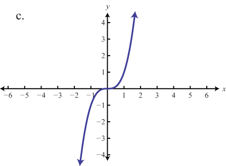
The cubing function47, defined by \(f (x) = x^{3}\), raises all of the values in the domain to the third power. The results can be either positive, zero, or negative. For example, \(f (1) = (1)^{3} = 1, f (0) = (0)^{3} = 0\), and \(f (−1) = (−1)^{3} = −1\).
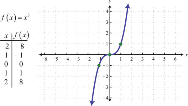
The domain and range both consist of all real numbers \(ℝ\).
Note that the constant, identity, squaring, and cubing functions are all examples of basic polynomial functions. The next three basic functions are not polynomials.
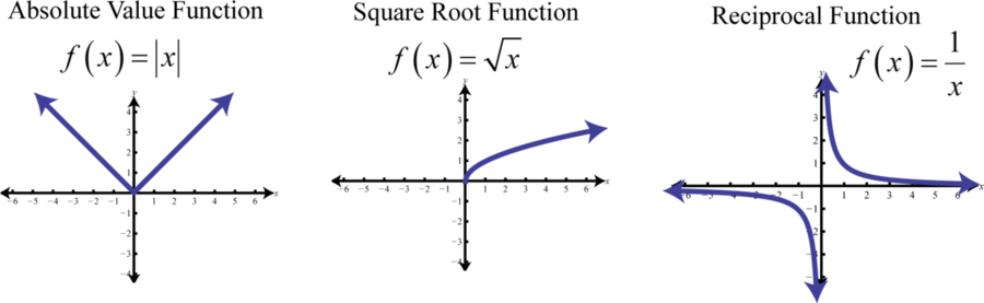
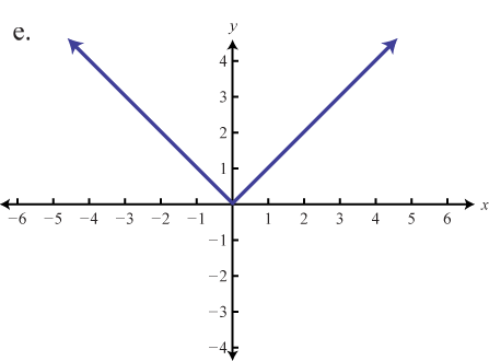
The absolute value function48, defined by \(f (x) = |x|\), is a function where the output represents the distance to the origin on a number line. The result of evaluating the absolute value function for any nonzero value of \(x\) will always be positive. For example, \(f (−2) = |−2| = 2\) and \(f (2) = |2| = 2\).
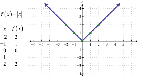
The domain of the absolute value function consists of all real numbers \(ℝ\) and the range consists of all \(y\)-values greater than or equal to zero \([0, ∞)\).
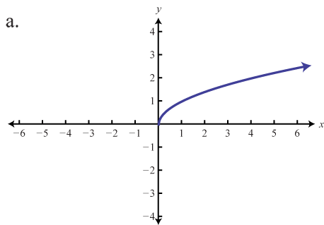
The square root function49, defined by \(f (x) = \sqrt{x}\), is not defined to be a real number if the \(x\)-values are negative. Therefore, the smallest value in the domain is zero. For example, \(f (0) = \sqrt{0}= 0\) and \(f (4) = \sqrt{4}= 2\).
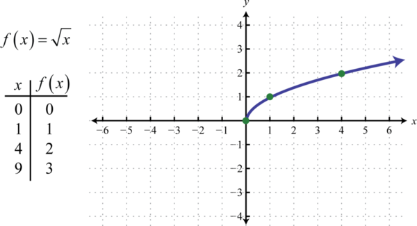
The domain and range both consist of real numbers greater than or equal to zero \([0, ∞)\).
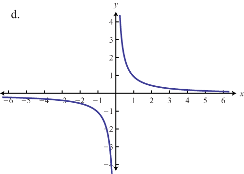
The reciprocal function50, defined by \(f (x) = \frac{1}{x}\), is a rational function with one restriction on the domain, namely \(x ≠ 0\). The reciprocal of an \(x\)-value very close to zero is very large. For example,
\(\begin{aligned} f ( 1 / 10 ) &= \frac { 1 } { \left( \frac { 1 } { 10 } \right) } = 1 \cdot \frac { 10 } { 1 } = 10 \\ f ( 1 / 100 ) &= \frac { 1 } { \left( \frac { 1 } { 100 } \right) } = 1 \cdot \frac { 100 } { 1 } = 100 \\ f ( 1 / 1,000 )& = \frac { 1 } { \left( \frac { 1 } { 1,000 } \right) } = 1 \cdot \frac { 1,000 } { 1 } = 1,000 \end{aligned}\)
In other words, as the \(x\)-values approach zero their reciprocals will tend toward either positive or negative infinity. This describes a vertical asymptote51 at the \(y\)-axis. Furthermore, where the \(x\)-values are very large the result of the reciprocal function is very small.
\(\begin{aligned} f ( 10 ) & = \frac { 1 } { 10 } = 0.1 \\ f ( 100 ) & = \frac { 1 } { 100 } = 0.01 \\ f ( 1000 ) & = \frac { 1 } { 1,000 } = 0.001 \end{aligned}\)
In other words, as the \(x\)-values become very large the resulting \(y\)-values tend toward zero. This describes a horizontal asymptote52 at the \(x\)-axis. After plotting a number of points the general shape of the reciprocal function can be determined.
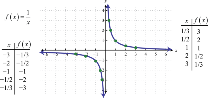
Both the domain and range of the reciprocal function consists of all real numbers except \(0\), which can be expressed using interval notation as follows: \((−∞, 0) ∪ (0, ∞)\).
In summary, the basic polynomial functions are:
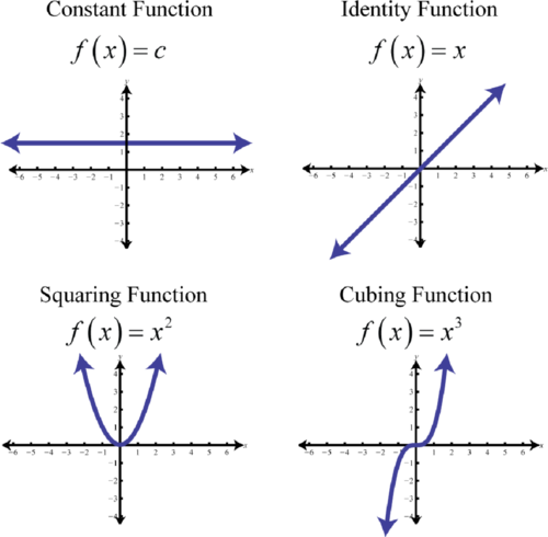
Figure \(\PageIndex{8}\)
The basic nonpolynomial functions are:
Piecewise Defined Functions
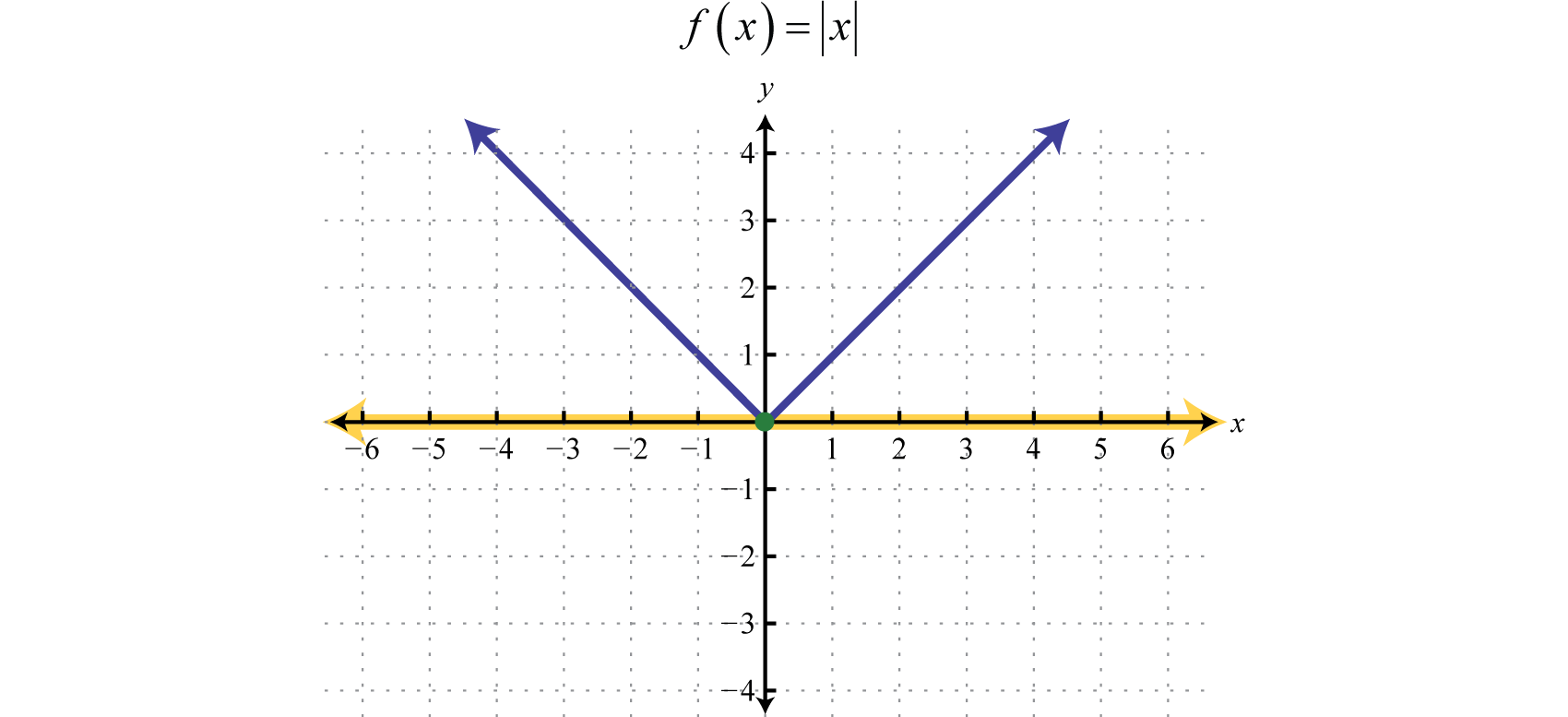
A piecewise function53, or split function54, is a function whose definition changes depending on the value in the domain. For example, we can write the absolute value function \(f(x) = |x|\) as a piecewise function:
\(f ( x ) = | x | = \left\{ \begin{array} { c l } { x } & { \text { if } x \geq 0 } \\ { - x } & { \text { if } x < 0 } \end{array} \right.\)
In this case, the definition used depends on the sign of the \(x\)-value. If the \(x\)-value is positive, \(x ≥ 0\), then the function is defined by \(f(x) = x\). And if the \(x\)-value is negative, \(x < 0\), then the function is defined by \(f(x) = −x\).
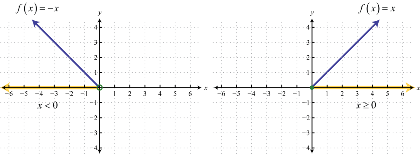
Following is the graph of the two pieces on the same rectangular coordinate plane:
Example \(\PageIndex{1}\):
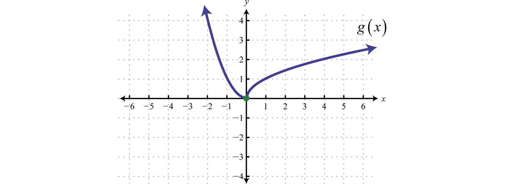
Graph: \(g ( x ) = \left\{ \begin{array} { c c c } { x ^ { 2 } } & { \text { if } } & { x < 0 } \\ { \sqrt { x } } & { \text { if } } & { x \geq 0 } \end{array} \right.\).
Solution
In this case, we graph the squaring function over negative \(x\)-values and the square root function over positive \(x\)-values.
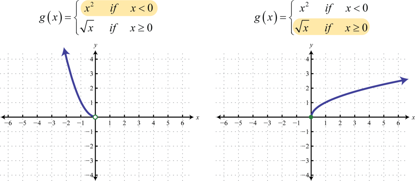
Notice the open dot used at the origin for the squaring function and the closed dot used for the square root function. This was determined by the inequality that defines the domain of each piece of the function. The entire function consists of each piece graphed on the same coordinate plane.
Answer:
When evaluating, the value in the domain determines the appropriate definition to use.
Example \(\PageIndex{2}\):
Given the function \(h\), find \(h(−5), h(0),\) and \(h(3)\).
Solution
Use \(h(t) = 7t + 3\) where \(t\) is negative, as indicated by \(t < 0\).
\(\begin{aligned} h ( t ) & = 7 t + 5 \\ h ( \color{Cerulean}{- 5}\color{Black}{ )} & = 7 ( \color{Cerulean}{- 5}\color{Black}{)} + 3 \\ & = - 35 + 3 \\ & = - 32 \end{aligned}\)
Where \(t\) is greater than or equal to zero, use \(h(t) = −16t^{2} + 32t\).
\(\begin{aligned} h ( \color{Cerulean}{0}\color{Black}{ )} & = - 16 ( \color{Cerulean}{0}\color{Black}{ )} + 32 ( \color{Cerulean}{0}\color{Black}{ )} h ( \color{Cerulean}{3}\color{Black}{ )} = 16 ( \color{Cerulean}{3}\color{Black}{ )} ^ { 2 } + 32 ( \color{Cerulean}{3}\color{Black}{ )} \\ & = 0 + 0 \quad\quad\quad\quad\quad\:\quad = -144 +96 \\ & = 0 \quad\quad\quad\quad\quad\quad\quad\quad = - 48 \end{aligned}\)
Answer:
\(h(−5) = −32, h(0) = 0,\) and \(h(3) = −48\)
Exercise \(\PageIndex{1}\)
Graph: \(f ( x ) = \left\{ \begin{array} { l l } { \frac { 2 } { 3 } x + 1 } & { \text { if } x < 0 } \\ { x ^ { 2 } } & { \text { if } x \geq 0 } \end{array} \right.\).
- Answer
-
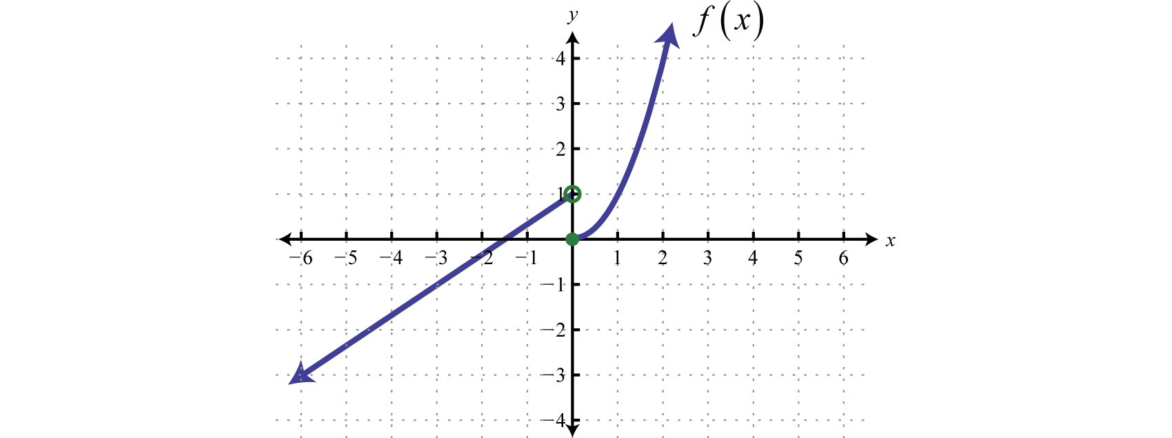
Figure \(\PageIndex{14}\) www.youtube.com/v/0hEUnSN5Blw
The definition of a function may be different over multiple intervals in the domain.
Example \(\PageIndex{3}\):
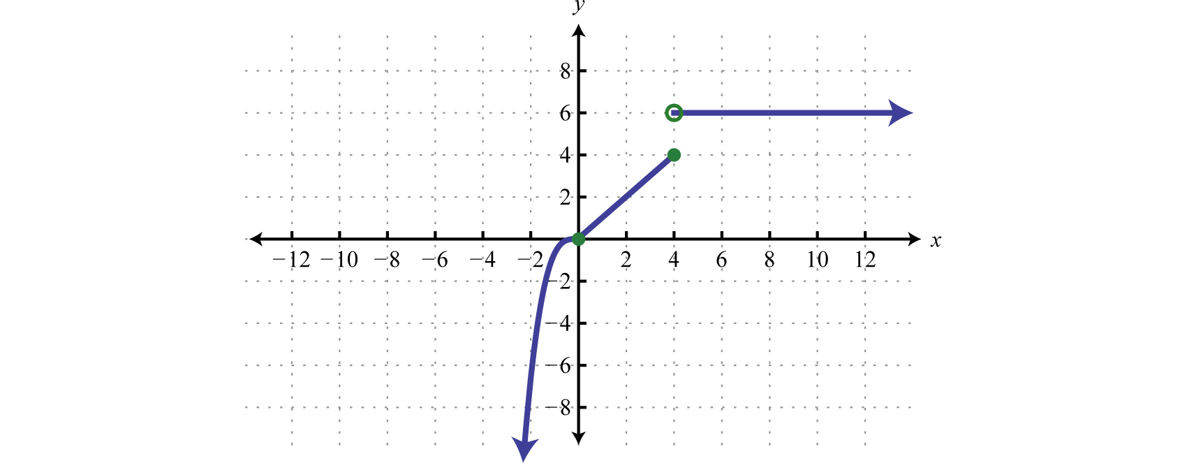
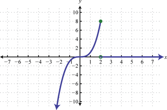
Graph: \(f ( x ) = \left\{ \begin{array} { l l } { x ^ { 3 } } & { \text { if } x < 0 } \\ { x } & { \text { if } 0 \leq x \leq 4 } \\ { 6 } & { \text { if } x > 4 } \end{array} \right.\).
Solution
In this case, graph the cubing function over the interval \((−∞,0)\). Graph the identity function over the interval \([0,4]\). Finally, graph the constant function \(f(x)=6\) over the interval \((4,∞)\). And because \(f(x)=6\) where \(x>4\), we use an open dot at the point \((4,6)\). Where \(x=4\), we use \(f(x)=x\) and thus \((4,4)\) is a point on the graph as indicated by a closed dot.
Answer:
The greatest integer function55, denoted \(f(x) = \left[\!\![x]\!\!\right]\), assigns the greatest integer less than or equal to any real number in its domain. For example,
\(\begin{aligned} f ( 2.7 ) & = \left[\!\![2.7]\!\!\right] = 2 \\ f ( \pi ) & = \left[\!\![\pi]\!\!\right] = 3 \\ f ( 0.23 ) & = \left[\!\![0.23]\!\!\right] = 0 \\ f ( - 3.5 ) & = \left[\!\![-3.5]\!\!\right] = - 4 \end{aligned}\)
This function associates any real number with the greatest integer less than or equal to it and should not be confused with rounding off.
Example \(\PageIndex{4}\):
Graph: \(f(x) = \left[\!\![x]\!\!\right]\).
Solution
If \(x\) is any real number, then \(y = \left[\!\![x]\!\!\right]\) is the greatest integer less than or equal to \(x\).
\(\begin{aligned} \vdots\\- 1 \leq x < 0 & \color{Cerulean}{\Rightarrow}\color{Black}{ y} = \left[\!\![x]\!\!\right] = -1 \\ 0 \leq x < 1 & \color{Cerulean}{\Rightarrow} \color{Black}{y} = \left[\!\![x]\!\!\right] = 0 \\ 1 \leq x < 2 & \color{Cerulean}{\Rightarrow}\color{Black}{ y} = \left[\!\![x]\!\!\right] = 1 \\ & \vdots \end{aligned}\)
Using this, we obtain the following graph.
Answer:
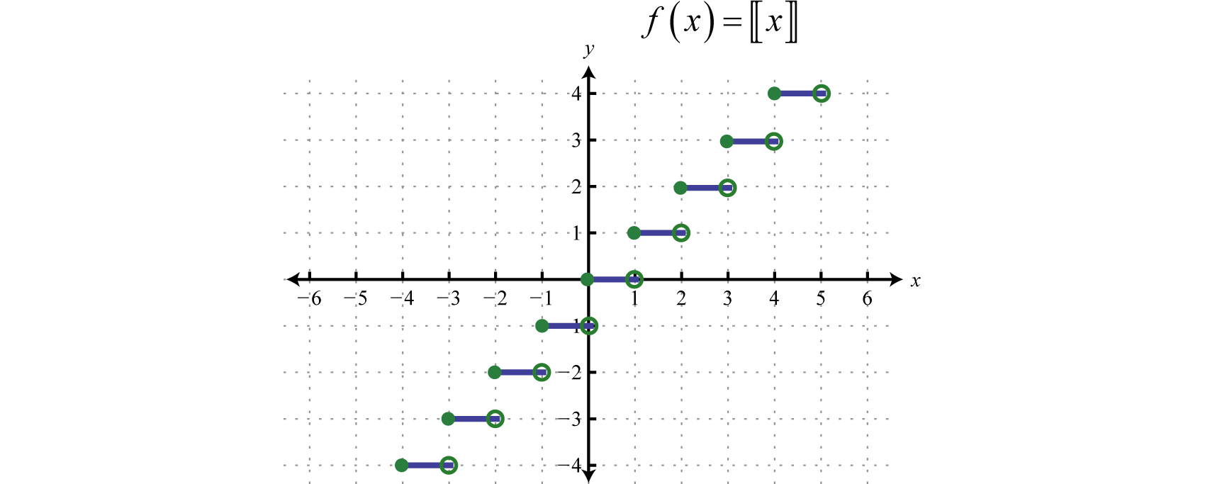
The domain of the greatest integer function consists of all real number \(\mathbb{R}\) and the range consists of the set of integers \(\mathbb{Z}\). This function is often called the floor function56 and has many applications in computer science.
Key Takeaways
- Plot points to determine the general shape of the basic functions. The shape, as well as the domain and range, of each should be memorized.
- The basic polynomial functions are: \(f(x) = c, f(x) = x , f(x) = x^{2}\), and \(f(x) = x^{3}\).
- The basic nonpolynomial functions are: \(f(x) = |x|, f(x) = \sqrt{x}\), and \(f(x) = \frac{1}{x}\).
- A function whose definition changes depending on the value in the domain is called a piecewise function. The value in the domain determines the appropriate definition to use.
Exercise \(\PageIndex{2}\)
Match the graph to the function definition.
- \(f(x) = x\)
- \(f(x) = x^{2}\)
- \(f(x) = x^{3}\)
- \(f(x) = |x|\)
- \(f(x) = x\)
- \(f(x) = \frac{1}{x}\)
- Answer
-
1. \(b\)
3. \(c\)
5. \(a\)
Exercise \(\PageIndex{3}\)
Evaluate.
- \(f(x) = x\); find \(f(−10), f(0)\), and \(f(a)\).
- \(f(x) = x^{2}\); find \(f(−10), f(0)\), and \(f(a)\).
- \(f(x) = x^{3}\); find \(f(−10), f(0)\), and \(f(a)\).
- \(f(x) = |x|\); find \(f(−10), f(0)\), and \(f(a)\).
- \(f(x) = \sqrt{x}\); \(find f(25), f(0)\), and \(f(a)\) where \(a ≥ 0\).
- \(f(x) = \frac{1}{x}\); find \(f(−10), f (\frac{1}{5})\), and \(f(a)\) where \(a ≠ 0\).
- \(f(x) = 5\); find \(f(−10), f(0)\), and \(f(a)\).
- \(f(x) = −12\); find \(f(−12), f(0)\), and \(f(a)\).
- Graph \(f(x) = 5\) and state its domain and range.
- Graph \(f(x) = −9\) and state its domain and range
- Answer
-
1. \(f ( - 10 ) = - 10 , f ( 0 ) = 0 , f ( a ) = a\)
3. \(f ( - 10 ) = - 1,000 , f ( 0 ) = 0 , f ( a ) = a ^ { 3 }\)
5. \(f ( 25 ) = 5 , f ( 0 ) = 0 , f ( a ) = \sqrt { a }\)
7. \(f ( - 10 ) = 5 , f ( 0 ) = 5 , f ( a ) = 5\)
9. Domain: \(\mathbb{R}\); range \(\{5\}\)
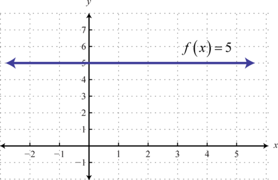
Figure \(\PageIndex{23}\)
Exercise \(\PageIndex{4}\)
Cube root function.
- 17. Find points on the graph of the function defined by \(f ( x ) = \sqrt [ 3 ] { x }\) with \(x\)-values in the set \(\{−8, −1, 0, 1, 8\}\).
- Find points on the graph of the function defined by \(f ( x ) = \sqrt [ 3 ] { x }\) with \(x\)-values in the set \(\{−3, −2, 1, 2, 3\}\). Use a calculator and round off to the nearest tenth.
- Graph the cube root function defined by \(f ( x ) = \sqrt [ 3 ] { x }\) by plotting the points found in the previous two exercises.
- Determine the domain and range of the cube root function.
- Answer
-
1. \(\{ ( - 8 , - 2 ) , ( - 1 , - 1 ) , ( 0,0 ) , ( 1,1 ) , ( 8,2 ) \}\)
3.
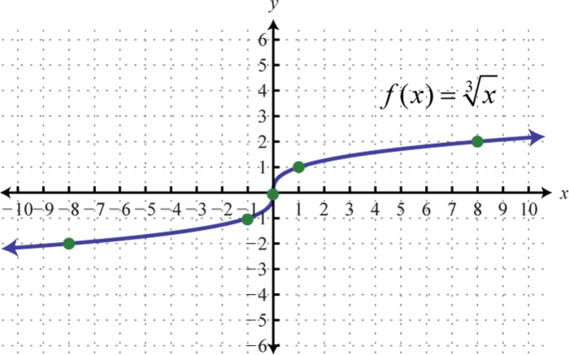
Figure \(\PageIndex{24}\)
Exercise \(\PageIndex{5}\)
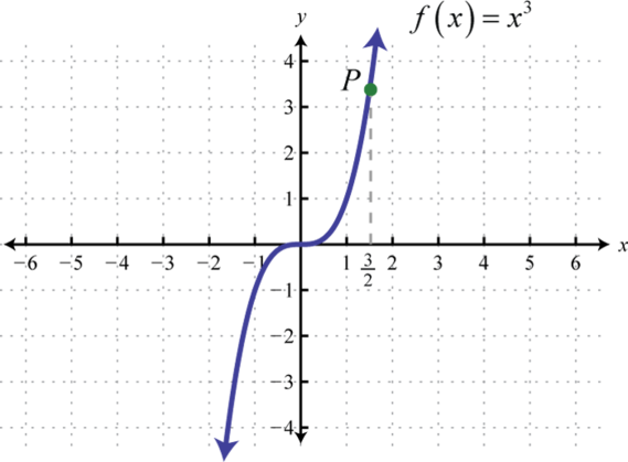
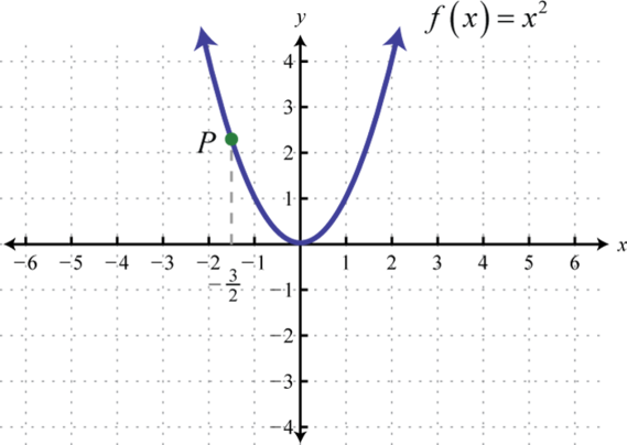
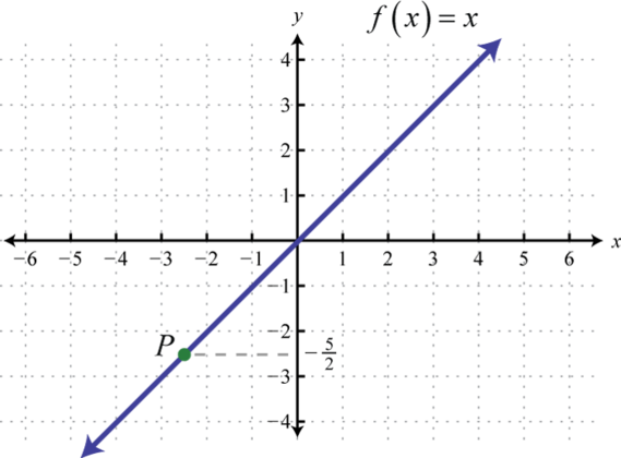
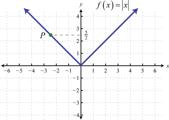
Find the ordered pair that specifies the point \(P\).
1.
2.
3.
4.
- Answer
-
1. \(\left( \frac { 3 } { 2 } , \frac { 27 } { 8 } \right)\)
3. \(\left( - \frac { 5 } { 2 } , - \frac { 5 } { 2 } \right)\)
Exercise \(\PageIndex{6}\)
Graph the piecewise functions.
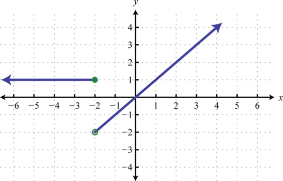
- \(g ( x ) = \left\{ \begin{array} { l l } { 2 } & { \text { if } x < 0 } \\ { x } & { \text { if } x \geq 0 } \end{array} \right.\)
- \(g ( x ) = \left\{ \begin{array} { l l } { x ^ { 2 } } & { \text { if } x < 0 } \\ { 3 } & { \text { if } x \geq 0 } \end{array} \right.\)
- \(h ( x ) = \left\{ \begin{array} { l l } { x } & { \text { if } x < 0 } \\ { \sqrt { x } } & { \text { if } x \geq 0 } \end{array} \right.\)
- \(h ( x ) = \left\{ \begin{array} { l } { | x | \text { if } x < 0 } \\ { x ^ { 3 } \text { if } x \geq 0 } \end{array} \right.\)
- \(f ( x ) = \left\{ \begin{array} { l } { | x | \text { if } x < 2 } \\ { 4 \text { if } x \geq 2 } \end{array} \right.\)
- \(f ( x ) = \left\{ \begin{array} { l l } { x } & { \text { if } x < 1 } \\ { \sqrt { x } } & { \text { if } x \geq 1 } \end{array} \right.\)
- \(g ( x ) = \left\{ \begin{array} { l l } { x ^ { 2 } \text { if } x \leq - 1 } \\ { x \quad \text { if } x > - 1 } \end{array} \right.\)
- \(g ( x ) = \left\{ \begin{array} { l } { - 3 \text { if } x \leq - 1 } \\ { x ^ { 3 } \text { if } x > - 1 } \end{array} \right.\)
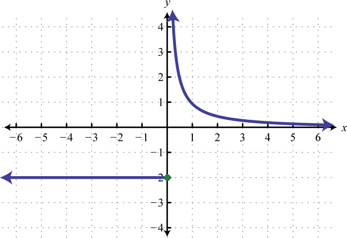
- \(h ( x ) = \left\{ \begin{array} { l } { 0 \text { if } x \leq 0 } \\ { \frac { 1 } { x } \text { if } x > 0 } \end{array} \right.\)
- \(h ( x ) = \left\{ \begin{array} { l } { \frac { 1 } { x } \text { if } x < 0 } \\ { x ^ { 2 } \text { if } x \geq 0 } \end{array} \right.\)
- \(f ( x ) = \left\{ \begin{array} { l l } { x ^ { 2 } } & { \text { if } x < 0 } \\ { x } & { \text { if } 0 \leq x < 2 } \\ { - 2 } & { \text { if } x \geq 2 } \end{array} \right.\)
- \(f ( x ) = \left\{ \begin{array} { l l } { x } & { \text { if } x < - 1 } \\ { x ^ { 3 } } & { \text { if } - 1 \leq x < 1 } \\ { 3 } & { \text { if } x \geq 1 } \end{array} \right.\)
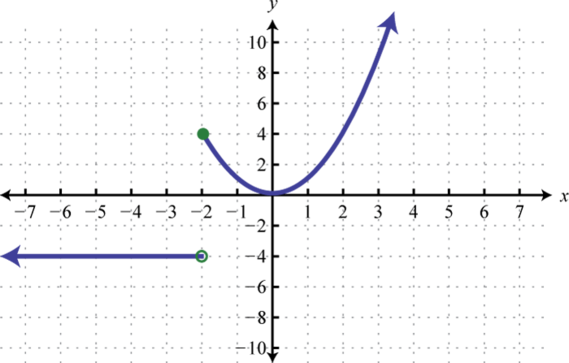
- \(g ( x ) = \left\{ \begin{array} { l l } { 5 } & { \text { if } x < - 2 } \\ { x ^ { 2 } } & { \text { if } - 2 \leq x < 2 } \\ { x } & { \text { if } x \geq 2 } \end{array} \right.\)
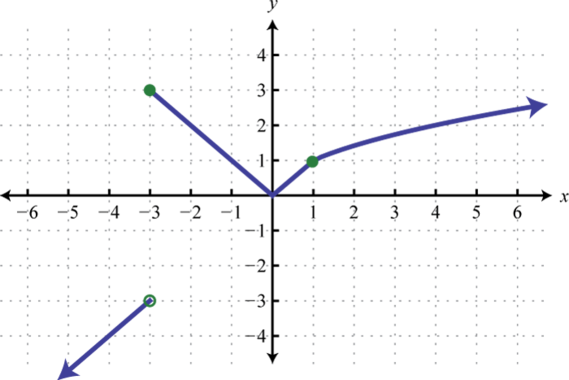
- \(g ( x ) = \left\{ \begin{array} { l l } { x } & { \text { if } x < - 3 } \\ { | x | } & { \text { if } - 3 \leq x < 1 } \\ { \sqrt { x } } & { \text { if } x \geq 1 } \end{array} \right.\)
- \(h ( x ) = \left\{ \begin{array} { l } { \frac { 1 } { x } \text { if } x < 0 } \\ { x ^ { 2 } \text { if } 0 \leq x < 2 } \\ { 4 \text { if } x \geq 2 } \end{array} \right.\)
- \(h ( x ) = \left\{ \begin{array} { l } { 0 \text { if } x < 0 } \\ { x ^ { 3 } \text { if } 0 < x \leq 2 } \\ { 8 \text { if } x > 2 } \end{array} \right.\)
- \(f ( x ) = [\left[\!\![x+0.5]\!\!\right]\)
- \(f(x) = \left[\!\![x]\!\!\right] +1\)
- \(f(x) = \left[\!\![0.5x]\!\!\right]\)
- \(f(x) = 2\left[\!\![x]\!\!\right]\)
- Answer
-
1.
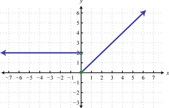
Figure \(\PageIndex{29}\) 3.
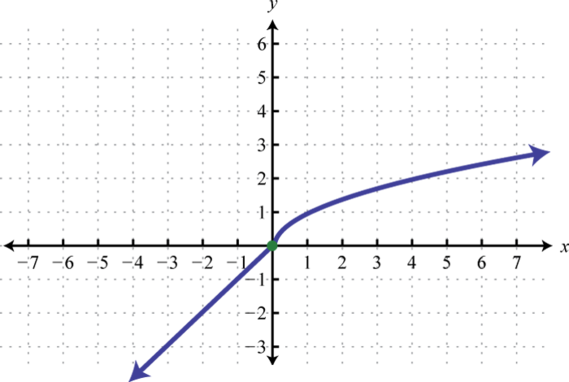
Figure \(\PageIndex{50}\) 5.
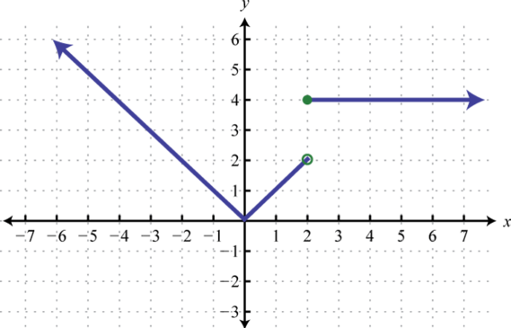
Figure \(\PageIndex{51}\) 7.
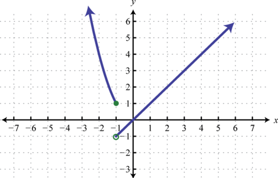
Figure \(\PageIndex{52}\) 9.
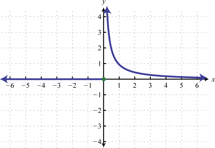
Figure \(\PageIndex{53}\) 11.
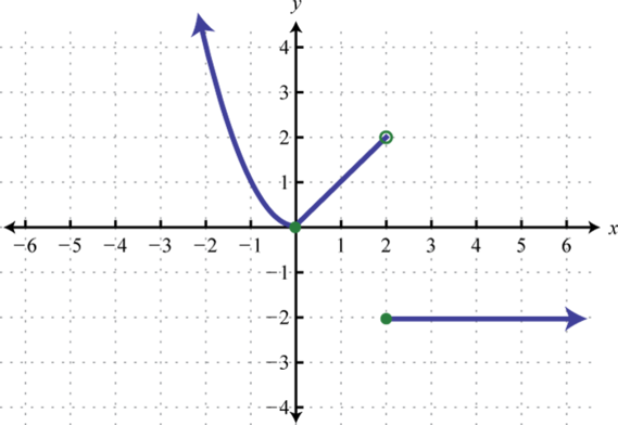
Figure \(\PageIndex{54}\) 13.
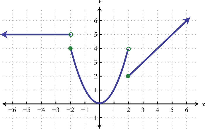
Figure \(\PageIndex{55}\) 15.
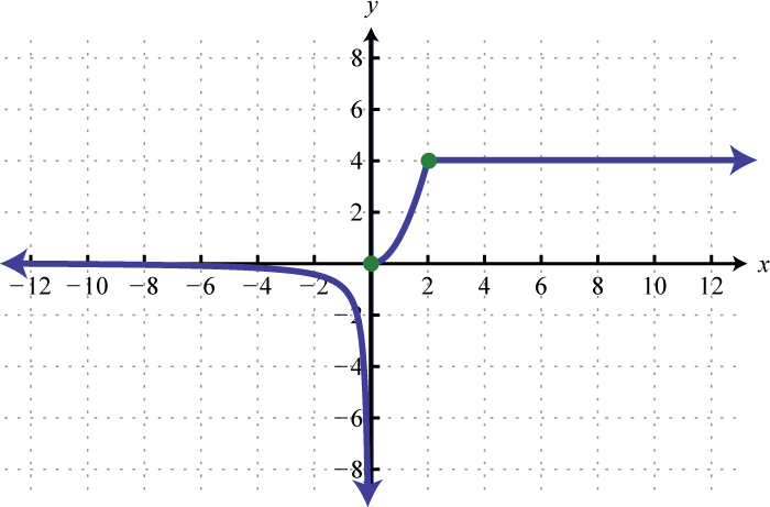
Figure \(\PageIndex{56}\) 17.
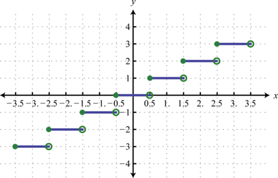
Figure \(\PageIndex{57}\) 19.
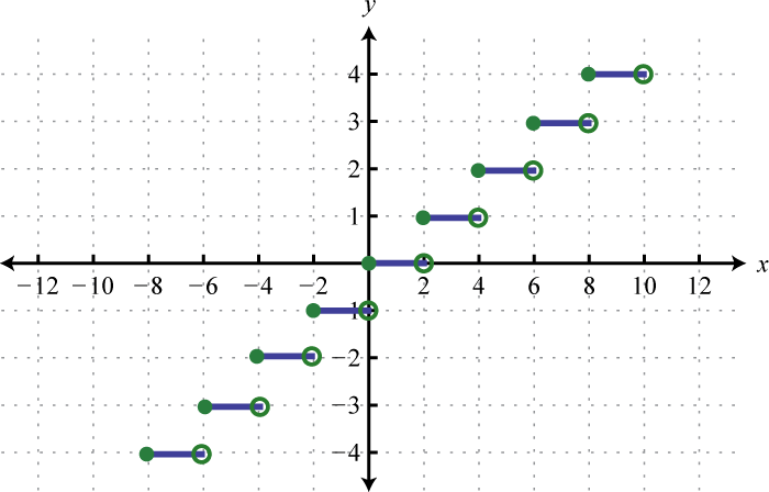
Figure \(\PageIndex{58}\)
Exercise \(\PageIndex{7}\)
Evaluate.
1. \(f ( x ) = \left\{ \begin{array} { l l } { x ^ { 2 } } & { \text { if } x \leq 0 } \\ { x + 2 } & { \text { if } x > 0 } \end{array} \right.\)
Find \(f(-5), f(0)\), and \(f(3)\).
2. \(f ( x ) = \left\{ \begin{array} { l l } { x ^ { 3 } } & { \text { if } x < 0 } \\ { 2 x - 1 } & { \text { if } x \geq 0 } \end{array} \right.\)
Find \(f(−3), f(0)\), and \(f(2)\).
3. \(g ( x ) = \left\{ \begin{array} { l l } { 5 x - 2 } & { \text { if } x < 1 } \\ { \sqrt { x } } & { \text { if } x \geq 1 } \end{array} \right.\)
Find \(g(−1), g(1)\), and \(g(4)\).
4. \(g ( x ) = \left\{ \begin{array} { l } { x ^ { 3 } \text { if } x \leq - 2 } \\ { | x | \text { if } x > - 2 } \end{array} \right.\)
Find \(g(−3), g(−2)\), and \(g(−1)\).
5. \(h ( x ) = \left\{ \begin{array} { l l } { - 5 } & { \text { if } x < 0 } \\ { 2 x - 3 } & { \text { if } 0 \leq x < 2 } \\ { x ^ { 2 } } & { \text { if } x \geq 2 } \end{array} \right.\)
Find \(h(−2), h(0)\), and \(h(4)\).
6. \(h ( x ) = \left\{ \begin{array} { l } { - 3 x \text { if } x \leq 0 } \\ { x ^ { 3 } \text { if } 0 < x \leq 4 } \\ { \sqrt { x } \text { if } x > 4 } \end{array} \right.\)
Find \(h(−5), h(4)\), and \(h(25)\).
7. \(f ( x ) = \left[\!\![x-0.5]\!\!\right]\)
Find \(f(−2), f(0)\), and \(f(3)\).
8. \(f ( x ) = \left[\!\![2x]\!\!\right] + 1\)
Find \(f(−1.2), f(0.4)\), and \(f(2.6)\).
- Answer
-
1. \(f (−5) = 25, f(0) = 0\), and \(f(3) = 5\)
3. \(g(−1) = −7, g(1) = 1\), and \(g(4) = 2\)
5. \(h(−2) = −5, h(0) = −3\), and \(h(4) = 16\)
7. \(f(−2) = −3, f(0) = −1\), and \(f(3) = 2\)
Exercise \(\PageIndex{8}\)
Evaluate given the graph of \(f\).
1. Find \(f(-4), f(-2)\), and \(f(0)\).
2. Find \(f(−3), f(0)\), and \(f(1)\).
3. Find \(f(0), f(2)\), and \(f(4)\).
4. Find \(f(−5), f(−2)\), and \(f(2)\).
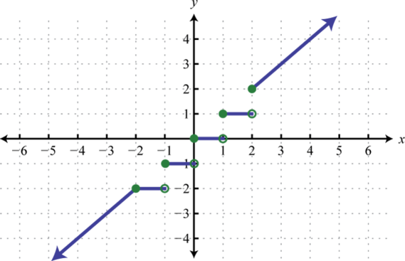
5. Find \(f(−3), f(−2)\), and \(f(2)\).
6. Find \(f(−3), f(0)\), and \(f(4)\).
7. Find \(f(−2), f(0)\), and \(f(2)\).
8. Find \(f(−3), f(1)\), and \(f(2)\).
9. The value of an automobile in dollars is given in terms of the number of years since it was purchased new in \(1975\):
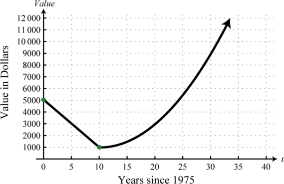
(1) Determine the value of the automobile in the year \(1980\).
(2) In what year is the automobile valued at \($9,000\)?
10. The cost per unit in dollars of custom lamps depends on the number of units produced according to the following graph:
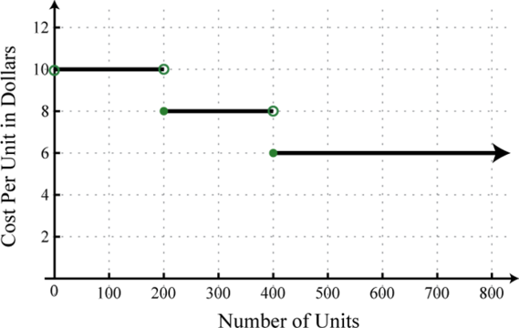
(1) What is the cost per unit if \(250\) custom lamps are produced?
(2) What level of production minimizes the cost per unit?
11. An automobile salesperson earns a commission based on total sales each month \(x\) according to the function:
\(( x ) = \left\{ \begin{array} { l l } { 0.03 x\quad \text { if } \quad 0 \leq x < \$ 20,000 } \\ { 0.05 x \quad\text { if } } \quad { \$ 20,000 \leq x < \$ 50,000 } \\ { 0.07 x \quad\text { if } }\quad { x \geq \$ 50,000 } \end{array} \right.\)
(1) If the salesperson’s total sales for the month are \($35,500\), what is her commission according to the function?
(2) To reach the next level in the commission structure, how much more in sales will she need?
12. A rental boat costs \($32\) for one hour, and each additional hour or partial hour costs \($8\). Graph the cost of the rental boat and determine the cost to rent the boat for \(4 \frac{1}{2}\) hours.
- Answer
-
1. \(f(−4) = 1, f(−2) = 1\), and \(f(0) = 0\)
3. \(f(0) = 0, f(2) = 8\), and \(f(4) = 0\)
5. \(f(−3) = 5, f(−2) = 4\), and \(f(2) = 2\)
7. \(f(−2) = −1, f(0) = 0\), and \(f(2) = 1\)
9. (1) \($3,000\); (2) \(2005\)
11. (1) \($1,775\); (2) \($14,500\)
Exercise \(\PageIndex{9}\)
- Explain to a beginning algebra student what an asymptote is.
- Research and discuss the difference between the floor and ceiling functions. What applications can you find that use these functions?
- Answer
-
1. Answer may vary
Footnotes
43Any function of the form \(f(x) = c\) where \(c\) is a real number.
44The linear function defined by \(f(x) = x\).
45The quadratic function defined by \(f(x) = x^{2}\).
46The curved graph formed by the squaring function.
47The cubic function defined by \(f(x) = x^{3}\).
48The function defined by \(f(x) = |x|\).
49The function defined by \(f(x) = \sqrt{x}\).
50The function defined by \(f(x) = \frac{1}{x}\).
51A vertical line to which a graph becomes infinitely close.
52A horizontal line to which a graph becomes infinitely close where the \(x\)-values tend toward \(±∞\).
53A function whose definition changes depending on the values in the domain.
54A term used when referring to a piecewise function.
55The function that assigns any real number \(x\) to the greatest integer less than or equal to \(x\) denoted \(f(x) = \left[\!\![x]\!\!\right]\).
56A term used when referring to the greatest integer function.