1.5: Quadratic Equations with Complex Roots

Last updated
Save as PDF

Page ID: 40893

$ \newcommand{\vecs}[1]{\overset { \scriptstyle \rightharpoonup} {\mathbf{#1}} } $ $ \newcommand{\vecd}[1]{\overset{-\!-\!\rightharpoonup}{\vphantom{a}\smash {#1}}} $$\newcommand{\id}{\mathrm{id}}$ $ \newcommand{\Span}{\mathrm{span}}$ $ \newcommand{\kernel}{\mathrm{null}\,}$ $ \newcommand{\range}{\mathrm{range}\,}$ $ \newcommand{\RealPart}{\mathrm{Re}}$ $ \newcommand{\ImaginaryPart}{\mathrm{Im}}$ $ \newcommand{\Argument}{\mathrm{Arg}}$ $ \newcommand{\norm}[1]{\| #1 \|}$ $ \newcommand{\inner}[2]{\langle #1, #2 \rangle}$ $ \newcommand{\Span}{\mathrm{span}}$ $\newcommand{\id}{\mathrm{id}}$ $ \newcommand{\Span}{\mathrm{span}}$ $ \newcommand{\kernel}{\mathrm{null}\,}$ $ \newcommand{\range}{\mathrm{range}\,}$ $ \newcommand{\RealPart}{\mathrm{Re}}$ $ \newcommand{\ImaginaryPart}{\mathrm{Im}}$ $ \newcommand{\Argument}{\mathrm{Arg}}$ $ \newcommand{\norm}[1]{\| #1 \|}$ $ \newcommand{\inner}[2]{\langle #1, #2 \rangle}$ $ \newcommand{\Span}{\mathrm{span}}$$\newcommand{\AA}{\unicode[.8,0]{x212B}}$

In Section $1.3,$ we considered the solution of quadratic equations that had two real-valued roots. This was due to the fact that in calculating the roots for each equation, the portion of the quadratic formula that is square rooted ($b^{2}-4 a c,$ often called the discriminant) was always a positive number.

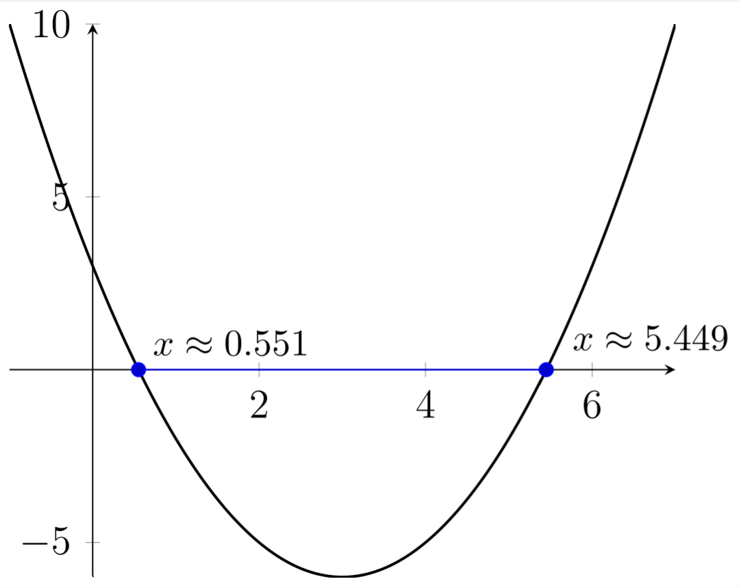
For example, in using the quadratic formula to calculate the the roots of the equation $x^{2}-6 x+3=0,$ the discriminant is positive and we will end up with two real-valued roots:
\[
\begin{array}{c}
x^{2}-6 x+3=0 \\
a=1, b=-6, c=3 \\
=\frac{-(-6) \pm \sqrt{(-6)^{2}-4(1)(3)}}{2 * 1} \\
=\frac{6 \pm \sqrt{36-12}}{2} \\
=\frac{6 \pm \sqrt{24}}{2} \\
=\frac{6 \pm 4.899}{2}
\end{array}
\]
\begin{array}{ll}
\approx \frac{6+4.899}{2} & \approx \frac{6-4.899}{2} \\
\approx \frac{10.899}{2} & \approx \frac{1.101}{2} \\
\approx 5.449 & \approx 0.551
\end{array}

When we added and subtracted the square root of 24 to 6 in the quadratic formula, this created two answers, and they were real-valued because the square root of 24 is real-valued.

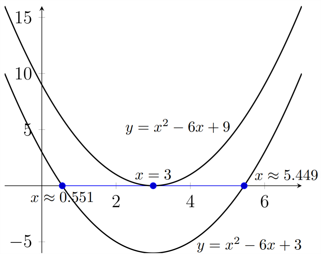
Another way to see this is graphically. If we graph $y=x^{2}-6 x+3$ and find the $x$ values that make $y=0,$ these will appear along the $x$ -axis, and will be the same values that solve the equation $x^{2}-6 x+3=0$

$clipboard_eab9383daac643dacd53365942d3a720e.png$

If we consider a related, but slightly different equation to start with, these relationships between the roots, the discriminant and the graphical intersections will be slightly different.
\[
\begin{array}{c}
x^{2}-6 x+9=0 \\
a=1, b=-6, c=9
\end{array}
\]

\begin{aligned}
x &=\frac{-(-6) \pm \sqrt{(-6)^{2}-4(1)(9)}}{2 * 1} \\
&=\frac{6 \pm \sqrt{36-36}}{2} \\
&=\frac{6 \pm \sqrt{0}}{2} \\
&=\frac{6}{2}=3
\end{aligned}

Because the discriminant was 0 in this problem, we only get one real-valued answer.

Graphically, the additional 6 that was added to the original equation to change it from $x^{2}-6 x+3$ to $x^{2}-6 x+9$ shifts every $y$ value on the graph up 6 units.

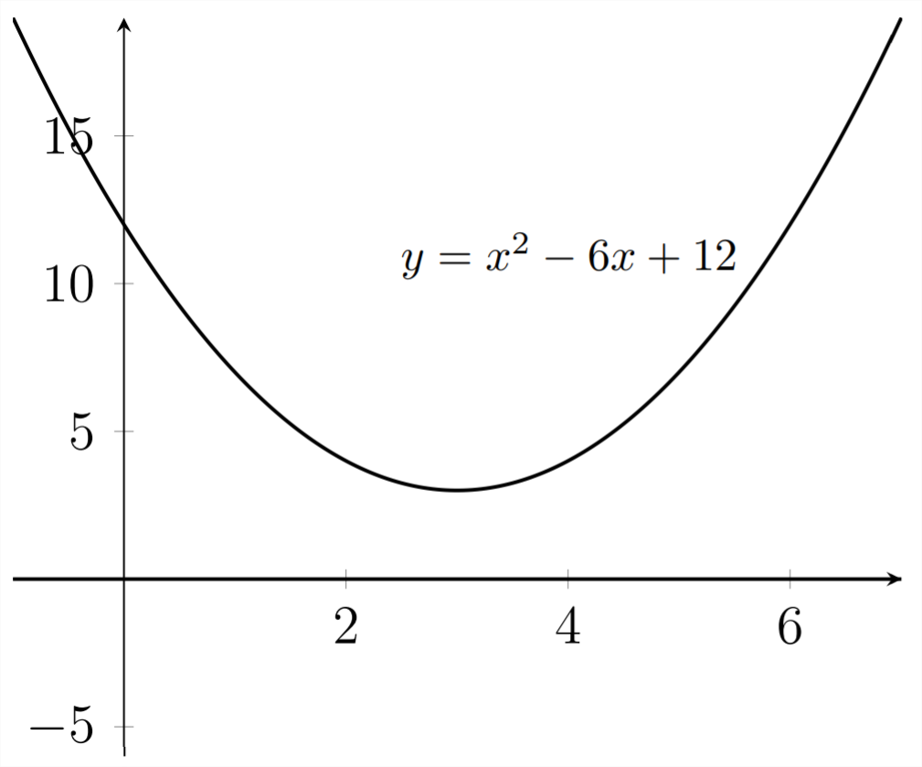
$clipboard_e9cfaae9a50287b0201636360c69e08b7.png$

If we add an additional three units to the constant term of this quadratic equation, we encounter a third possibility.

\begin{array}{c}
x^{2}-6 x+12=0 \\
a=1, b=-6, c=12 \\
=\frac{-(-6) \pm \sqrt{(-6)^{2}-4(1)(12)}}{2 * 1} \\
=\frac{6 \pm \sqrt{36-48}}{2} \\
=\frac{6 \pm \sqrt{-12}}{2} \\
=\frac{6}{2} \pm \frac{6 \cdot 464 i}{2} \\
\approx 3 \pm 1.732 i
\end{array}

Here the discriminant is negative, which leads to two complex-valued answers. If the equation has real-valued coefficients, the complex roots will always come in conjugate pairs. Complex conjugates share the same real-valued part and have opposite signs in their complex-valued (or imaginary) parts: $a \pm b i$

Graphically, the previous problem was one step away from not intersecting the $x$ -axis at all and the additional three units that we added on to get $y=x^{2}-$ $6 x+12$ moves the graph entirely away from the $x$ -axis. Because the roots are complex-valued, we don't see any roots on the $x$ -axis. The $x$ -axis contains only real numbers.

$clipboard_ed90c780180cc23c80ff55717aa7f2b1b.png$

since the calculator has been programmed for the quadratic formula, the focus of the problems in this section will be on putting them into standard form.

Example $\PageIndex{1}$

Solve for $x$
$(2 x+1)(x+5)-2 x(x+7)=5(x+3)^{2}$

Solution

\[
\begin{array}{c}
(2 x+1)(x+5)-2 x(x+7)=5(x+3)^{2} \\
2 x^{2}+11 x+5-2 x^{2}-14 x=5(x+3)(x+3) \\
-3 x+5=5\left(x^{2}+6 x+9\right) \\
-3 x+5=5 x^{2}+30 x+45 \\
0=5 x^{2}+33 x+40 \\
x=5, b=33, c=40 \\
x=-5,-1.6
\end{array}
\]

The fact that the roots of this equation were rational numbers means that the equation could have been solved by factoring.
\[
\begin{array}{cc}
0=5 x^{2}+33 x+40 \\
0=(5 x+8)(x+5) \\
5 x=-8 & x+5=0 \\
5 x+8=0 & x=-5 \\
x=-1.6 &
\end{array}
\]

Example $\PageIndex{1}$

Solve for $x$
$(x-2)^{2}+3(4 x-1)(x+1) &=7(x+1)(x-1)$

Solution

\[
\begin{aligned}
x^{2}-4 x+4+3\left(4 x^{2}+3 x-1\right) &=7\left(x^{2}-1\right) \\
x^{2}-4 x+4+12 x^{2}+9 x-3 &=7 x^{2}-7 \\
13 x^{2}+5 x+1 &=7 x^{2}-7 \\
6 x^{2}+5 x+8 &=0 \\
a=6, b=5, c=8 & \\
x \approx-0.41 \overline{6} \pm 1.077 i \approx-\frac{5}{12} \pm 1.077 i
\end{aligned}
\]

Exercise $\PageIndex{1}$

Solve for $x$ in each equation. Round any irrational values to the nearest 1000 th.
1) $\quad 3 x^{2}-3 x=4$
2) $\quad 4 x^{2}-2 x=7$
3) $\quad 5 x^{2}=3-7 x$
4) $\quad 3 x^{2}=21-14 x$
5) $\quad 6 x^{2}+1=2 x$
6) $\quad 5 x-3 x^{2}=17$
7) $\quad (5 x-1)(2 x+3)=3 x-20$
8) $\quad (x+4)(3 x-1)=9 x-5$
9) $\quad (x-2)^{2}=8 x(x-1)+10$
10) $\quad (2 x-3)^{2}=2 x-7 x^{2}$
11) $\quad (x+5)(x-6)=(2 x-1)(x-4)$
12) $\quad (3 x-4)(x+2)=(2 x-5)(x+5)$

Answer: 1) $\quad x \approx 1.758,-0.758$
3) $\quad x \approx 0.344,-1.744$
5) $\quad x \approx 0.1 \overline{6} \pm 0.373 i$
7) $\quad x \approx-0.5 \pm 1.204 i$
9) $\quad x \approx 0.286 \pm 0.881 i$
11) $\quad x \approx 4 \pm 4.243 i$