5.4: Library of functions

Knowing graphs of common functions assist the student with visualizing the function and connecting the relationship between the equation and its graph.

Library of Functions

The library of functions is a set of functions that distinguishes the relationship between the functions and their graphs which includes the domain for each function.

The library of functions grows as we become more familiar with different types of functions. As we take more higher-level mathematics, the library grows to be very large, but for this section, we begin with a library that contains six important basic functions: line, parabola, cubic, absolute value, rational, square root.

Note

The graphs of the functions in the library of functions are the general graphs of the functions, not particular graphs of functions. Hence, we can use point-plotting, technology, or transformations to graph particular functions, but we tend to memorize the general form as it is helpful in higher-level mathematics to recall the library of functions quickly.

Example 5.4.1

Graph \(f(x) = x\), \(g(x) = 2\), and \(h(x) = −3x + 1\) and determine their domain.

Solution

Notice, all three functions are linear functions. We can plot them easily on the same grid. We can see that all graphs are lines and since there are no restrictions to any of the lines, the domain is all real numbers or \((−∞, ∞)\). Since \(f\) is a line through the origin (\(y\)-intercept is zero), and every \(x\) coordinate is the same as its corresponding \(y\) coordinate, e.g., \((0, 0),\: (1, 1),\) etc., then we call \(f\) the identity function.

Figure 5.4.1

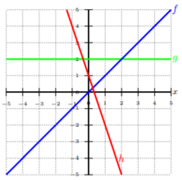
Since \(g\) is a horizontal line, the \(y\) coordinates never change, and there isn’t a change in slope, i.e., the slope is zero, then we call \(g\) the constant function.

The function \(h\) is an equation of a line with a nonzero slope and non-zero \(y\)-intercept, and we call \(h\) a linear function.

Example 5.4.2

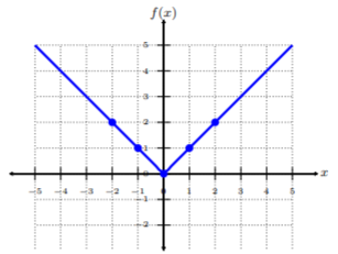
Graph \(f(x) = |x|\) and determine the domain.

Solution

Let’s pick five \(x\)-coordinates, and find corresponding \(y\)-values. Each \(x\)-value being positive or negative, and zero. This is common practice, but not required.

Table 5.4.1

\(x\)	\(f(x)=|x|\)	\((x,f(x))\)
\(-2\)	\(f(\color{blue}{-2}\color{black}{})=2\)	\((-2,2)\)
\(-1\)	\(f(\color{blue}{-1}\color{black}{})=1\)	\((-1,1)\)
\(0\)	\(f(\color{blue}{0}\color{black}{})=0\)	\((0,0)\)
\(1\)	\(f(\color{blue}{1}\color{black}{})=1\)	\((1,1)\)
\(2\)	\(f(\color{blue}{2}\color{black}{})=2\)	\((2,2)\)

Plot the five ordered-pairs from the table. To connect the points, be sure to connect them from smallest \(x\)-value to largest \(x\)-value, i.e., left to right. This graph looks like two lines of opposite slopes that meet at the origin. Hence, it’s graph is two lines that meet at the origin, but stop where it meets to make a v-shape called an absolute value function Since we see there are no restrictions to the graph, the domain is all real numbers or \((−∞, ∞)\).

Figure 5.4.2

Example 5.4.3

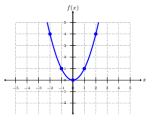
Graph \(f(x) = x^2\) and determine the domain.

Solution

Let’s pick five \(x\)-coordinates, and find corresponding \(y\)-values. Each \(x\)-value being positive, negative, and zero. This is common practice, but not required.

Table 5.4.2

\(x\)	\(f(x)=x^2\)	\((x,f(x)\)
\(-2\)	\(f(\color{blue}{-2}\color{black}{})=4\)	\((-2,4)\)
\(-1\)	\(f(\color{blue}{-1}\color{black}{})=1\)	\((-1,1)\)
\(0\)	\(f(\color{blue}{0}\color{black}{})=0\)	\((0,0)\)
\(1\)	\(f(\color{blue}{1}\color{black}{})=1\)	\((1,1)\)
\(2\)	\(f(\color{blue}{2}\color{black}{})=4\)	\((2,4)\)

Plot the five ordered-pairs from the table. To connect the points, be sure to connect them from smallest \(x\)-value to largest \(x\)-value, i.e., left to right. This graph is called a parabola and since this function is quite common for the \(x^2\)-form, we call it a quadratic (square) function. Since we see there are no restrictions to the graph, the domain is all real numbers or \((−∞, ∞)\).

Figure 5.4.3

Example 5.4.4

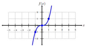
Graph \(f(x) = x^3\) and determine the domain.

Solution

Let’s pick three \(x\)-coordinates, and find corresponding \(y\)-values. Each \(x\)-value being positive, negative, and zero. This is common practice, but not required.

Table 5.4.3

\(x\)	\(f(x)=x^3\)	\((x,f(x))\)
\(-1\)	\(f(\color{blue}{-1}\color{black}{})=-1\)	\((-1,-1)\)
\(0\)	\(f(\color{blue}{0}\color{black}{})=0\)	\((0,0)\)
\(1\)	\(f(\color{blue}{1}\color{black}{})=1\)	\((1,1)\)

Plot the ordered-pairs from the table. To connect the points, be sure to connect them from smallest \(x\)-value to largest \(x\)-value, i.e., left to right. Since this function is quite common for the \(x^3\)-form, we call it a cube (cubic) function. Since we see there are no restrictions to the graph, the domain is all real numbers or \((−∞, ∞)\).

Figure 5.4.4

Example 5.4.5

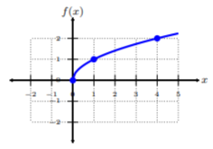
Graph \(f(x) =\sqrt{x}\) and determine the domain.

Solution

Let’s pick three \(x\)-coordinates, and find corresponding \(y\)-values.

Table 5.4.4

\(x\)	\(f(x)=\sqrt{x}\)	\((x,f(x))\)
\(0\)	\(f(\color{blue}{0}\color{black}{})=0\)	\((0,0)\)
\(1\)	\(f(\color{blue}{1}\color{black}{})=1\)	\((1,1)\)
\(4\)	\(f(\color{blue}{4}\color{black}{})=2\)	\((4,2)\)

Plot the ordered-pairs from the table. To connect the points, be sure to connect them from smallest \(x\)-value to largest \(x\)-value, i.e., left to right. Since this function is quite common for the \(\sqrt{x}\)-form, we call it a square root function. Since we see there is one restriction to the graph, where the \(x\) values start at the origin and no part of the graph is on the left side of the origin, the domain of this function is \(\{x|x ≥ 0\}\) or \([0, ∞)\).

Figure 5.4.5

Example 5.4.6

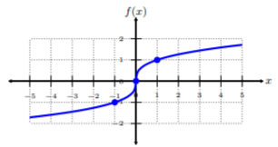
Graph \(f(x) =\sqrt[3]{x}\) and determine the domain.

Solution

Let’s pick three \(x\)-coordinates, and find corresponding \(y\)-values.

Table 5.4.5

\(x\)	\(f(x)=\sqrt[3]{x}\)	\((x,f(x))\)
\(-1\)	\(f(\color{blue}{-1}\color{black}{})=-1\)	\((-1,-1)\)
\(0\)	\(f(\color{blue}{0}\color{black}{})=0\)	\((0,0)\)
\(1\)	\(f(\color{blue}{1}\color{black}{})=1\)	\((1,1)\)

Plot the ordered-pairs from the table. To connect the points, be sure to connect them from smallest \(x\)-value to largest \(x\)-value, i.e., left to right. This function looks like the cube function, but flipped and \(90^{\circ}\) to the right! We call this function a cube root function. because of the root on the radical. Since we see there are no restrictions to the graph, the domain is all real numbers or \((−∞, ∞)\).

Figure 5.4.6

Example 5.4.7

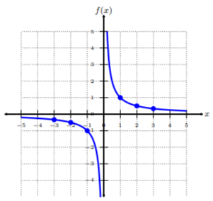
Graph \(f(x) =\dfrac{1}{x}\) and determine the domain.

Solution

Let’s pick \(x\)-coordinates, and find corresponding \(y\)-values.

Table 5.4.6

\(x\)	\(f(x)=\dfrac{1}{x}\)	\((x,f(x))\)
\(-3\)	\(f(\color{blue}{-3}\color{black}{})=-\dfrac{1}{3}\)	\((-3,-\dfrac{1}{3})\)
\(-2\)	\(f(\color{blue}{-2}\color{black}{})=-\dfrac{1}{2}\)	\((-2,-\dfrac{1}{2})\)
\(-1\)	\(f(\color{blue}{-1}\color{black}{})=-1\)	\((-1,-1)\)
\(0\)	\(f(\color{blue}{0}\color{black}{})=\text{undefined}\)	no point
\(1\)	\(f(\color{blue}{1}\color{black}{})=1\)	\((1,1)\)
\(2\)	\(f(\color{blue}{2}\color{black}{})=\dfrac{1}{2}\)	\((2,\dfrac{1}{2})\)
\(3\)	\(f(\color{blue}{3}\color{black}{})=\dfrac{1}{3}\)	\((3,\dfrac{1}{3})\)

Plot the ordered-pairs from the table. To connect the points, be sure to connect them from smallest \(x\)-value to largest \(x\)-value, i.e., left to right. This graph looks most different than the other functions and it is because it is a fraction with a variable in the denominator. Recall, fractions cannot have zero in their denominators because that is when fractions are undefined. We will learn more about these functions that are called rational functions. For now, we call the graph of this function a reciprocal function. Since we see that this function cannot have zero in the denominator, and, from the table, we see when \(x = 0\), the function is undefined, then the domain is all real numbers except for \(x = 0: \{x|x \neq 0\}\) or \((−∞, 0) ∪ (0, ∞)\).

Figure 5.4.7

Library of Functions Homework

Given below are the graphs of functions.

Figure 5.4.8

Exercise 5.4.1

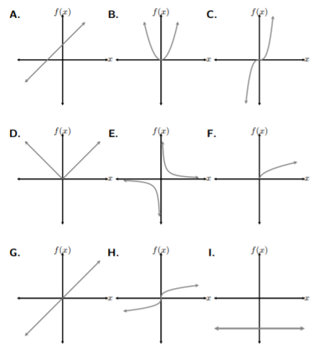
Match each graph with the name of its function.

Names of the Functions

1. Reciprocal Function
2. Absolute Value Function
3. Cube Root Function
4. Cube Function
5. Constant Function
6. Identity Function
7. Square Root Function
8. Square Function
9. Linear Function

Exercise 5.4.2

Match each graph with the formula of the function.

Formulas of Functions

1. \(f(x) = x\)
2. \(f(x) = −4\)
3. \(f(x) = |x|\)
4. \(f(x) = x^2\)
5. \(f(x) =\dfrac{1}{x}\)
6. \(f(x) = x^3\)
7. \(f(x) = mx + b\)
8. \(f(x) =\sqrt[3]{x}\)
9. \(f(x) =\sqrt{x}\)

Exercise 5.4.3

What are the domains for each of the functions?