
12.1: Inverse functions
- Page ID
- 45117

One-to-One Functions
Let’s begin by discussing the relationship of one-to-one. One-to-one functions are special functions where all the inputs and outputs of a function are distinct, i.e., none of the \(x\) or \(y\) coordinates repeat.
A function is one-to-one if any two different inputs in the domain correspond to two different outputs in the range, i.e., \(f(x_1)\neq f(x_2)\) for any \(x_1\) and \(x_2\).
Another way of determining one-to-one is to make sure all x and all y values are different.
Determine if the following relation is one-to-one.
\[\{(3,-5), (2,-1), (1,0), (0,7), (-1,8)\}\nonumber\]
Solution
We first look at all the inputs and outputs. By the definition, we need to make sure no \(x\) or \(y\) values repeat, i.e., all \(x\) and \(y\) coordinates are unique. We have
\[x\text{ − values }=3,2,1,0,-1\nonumber\]
and
\[y\text{ − values }=-5,-1,0,7,8\nonumber\]
Hence, none of the coordinates repeat, which means this relation is one-to-one.
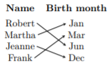
Determine if the following relation is one-to-one.
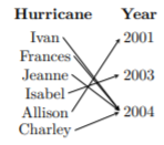
Solution
We first look at all the inputs and outputs. Let’s assume the name of the hurricane is the input and the year the hurricane took place is the output. By the definition, we need to make sure no \(x\) or \(y\) values repeat, i.e., all \(x\) and \(y\) coordinates are unique. We have
\[x \text{− values }=\text{ Ivan, Frances, Jeanne, Isabel, Allison, Charley}\nonumber\]
and
\[y\text{ − values }= 2004, 2004, 2004, 2003, 2001, 2004\nonumber\]
Hence, none of the \(x\) coordinates repeat, but the year 2004 repeats itself 4 times in the \(y\)-coordinates, which means this relation is not one-to-one.
The notation used for functions was first introduced by the great Swiss mathematician, Leonhard Euler, in the 18th century.
There is a graphical way to determine whether a given graph of a function is one-to-one and that is by the horizontal line test. As we used the vertical line test to determine whether a graph is a function, we use the horizontal line test to determine whether a graph of a function is one-to-one.
If every horizontal line intersects the graph of a function \(f\) at most one point, then \(f\) is one-to one.
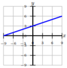
Determine which graphs of the functions below are one-to one.
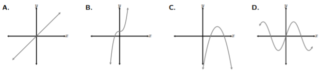
Solution
Let’s start by drawing horizontal lines throughout each graph and determine whether the line intersects the graph more than once. Now, recall, it is given that these graphs are all functions. Meaning, we assume all four of these functions have passed the vertical line test. We just need to see whether these functions are one-to-one by applying the horizontal line test.
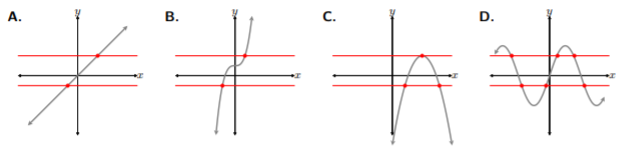
Looking at A. and B., we see that the horizontal lines intersect the graphs only once, passing the horizontal line test. If we take a look at C., the top line intersects the graph once because it is only intersecting at the parabola’s vertex, but looking at the bottom line, we see the horizontal line intersects the parabola two times. Hence, C. doesn’t pass the horizontal line test. Lastly, D. has both of its horizontal lines intersecting the graph more than once and resulting in failing the horizontal line test. Thus, graphs A. and B. both pass the horizontal line test and are one-to-one functions.
Be sure to draw complete horizontal lines, from left to right, filling the grid, and more than one. It is easy to draw a line and stop midway to conclude the graph passes the horizontal line test, like in C.. However, for the validity of the horizontal line test, we must draw complete horizontal lines, left to right, filling the grid, and more than one.
A Function and its Inverse
If \(f(x)\) is one-to-one, we call \(f(x)\) an invertible function with ordered pairs \((a, b)\). The inverse function, \(f^{−1} (x)\), is the set of ordered pairs \((b, a)\), i.e., \(y\)-coordinates and \(x\)-coordinates switch.
Find the inverse of the one-to-one function
\[\{(3, −1),(2, 7),(1, −4),(0, 8),(−1, 5)\}\nonumber\]
State the domain and range of the inverse function.
Solution
To find the inverse of a given one-to-one function, we need to identify all \(x\) and \(y\) coordinates and reverse them, i.e., by the definition, \(y\)-coordinates and \(x\)-coordinates switch. Let \(f(x) = \{(3, −1),(2, 7),(1, −4),(0, 8),(−1, 5)\}\). Then
\[f^{−1} (x) = \{(−1, 3),(7, 2),(−4, 1),(8, 0),(5, −1)\}\nonumber\]
The domain of \(f^{−1} (x)\) is \(\{−4, −1, 5, 7, 8\}\) and the range is \(\{−1, 0, 1, 2, 3\}\).
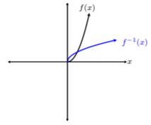
Draw the inverse function of the given one-to-one function.
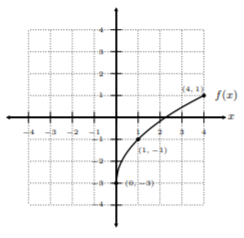
Solution
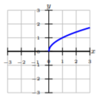
Using the same rationale as we did for Example 12.1.4 , we can take the well-defined ordered pairs on the graph of \(f(x)\) and switch the \(x\) and \(y\)-coordinates. Let’s place the ordered-pairs on a table:
\[\begin{array}{c|c} x & f(x)\\ \hline 0&-3 \\ 1&-1 \\ 4&1\end{array}\quad\text{this implies that }f^{-1}(x)\text{ is}\quad\begin{array}{c|c} x&f^{-1}(x) \\ \hline -3&0 \\ -1&1 \\ 1&4\end{array}\nonumber\]
Notice, all we did was switch the \(x\) and \(y\)-coordinates from the first table to obtain three well-defined ordered pairs on \(f^{−1} (x)\). Let’s graph these points and connect them with a nice smooth curve:
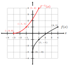
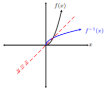
We can see from Example 12.1.5 , that the idea behind invertible functions is that \(x\) and \(y\) coordinates switch. In fact, if we look even closer at Example 12.1.5 ’s graph of \(f(x)\) and \(f^{−1} (x)\), we can see that \(f^{−1} (x)\) is a mirror image of \(f(x)\) about the line \(y = x\). Let’s draw the line \(y = x\) on the graph in Example 12.1.5 :
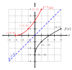
Hence, the line \(y = x\) acts like a mirror, and \(f(x)\) and \(f^{−1} (x)\) are reflections of each other about the line \(y = x\). This is no coincidence!
Recall. The definition of a composition of two functions.
Let \(f\) and \(g\) be functions of \(x\). If \(f\) is composed of \(g\), then
\[(f\circ g)(x)=f(g(x))\nonumber\]
We say \(f\) is composed of \(g\), i.e, we substitute every \(x\) in \(f\) with the function \(g(x)\).
\((f\circ g)(x)\) implies that \(x\) is in the domain of \(g(x)\) and \(g(x)\) is in the domain of \(f(x)\).
We can easily verify whether two functions are inverses of each other by using the property of the composition of \(f(x)\) and \(f^{−1} (x)\).
Given a function \(f(x)\) to be one-to-one, and \(f^{−1} (x)\) is \(f(x)\)’s inverse function, then
\[f(f^{-1}(x))=f^{-1}(f(x))=x\nonumber\]
Are \(f(x)=\sqrt[3]{3x+4}\) and \(g(x)=\dfrac{x^3-4}{3}\) inverses?
Solution
From the property above, we can use the composition of \(f\) and \(g\) to verify whether \(f(g(x))=x\). Recall, if \(f(g(x))=x\), then \(f\) and \(g\) are inverses.
\[\begin{aligned}f(\color{blue}{g(x)}\color{black}{)}&=f\left(\color{blue}{\dfrac{x^3-4}{3}}\right) \\ &=\sqrt[3]{\color{black}{\cancel{\color{red}{3}}}\left(\dfrac{x^3-4}{\color{black}{\cancel{\color{red}{3}}}}\right)+4} \\ &=\sqrt[3]{x^3-4+4} \\ &=\sqrt[3]{x^3} \\ &=x\end{aligned}\]
Notice, when we simplified \(f(g(x))\), we obtained the simplified expression \(x\), i.e.,
\[f(g(x))=x\nonumber\]
Thus, \(f(x)\) and \(g(x)\) are inverses of each other. We leave verifying \(g(f(x)) = x\) to the student.
Are \(h(x)=2x+5\) and \(g(x)=\dfrac{x}{2}-5\) inverses?
Solution
We can use the composition of \(h\) and \(g\) to verify whether \(h(x)\) and \(g(x)\) are inverses. Recall, if \(h(g(x))=x\), then \(h\) and \(g\) are inverses.
\[\begin{aligned}h(\color{blue}{g(x)})&=h\left(\color{blue}{\dfrac{x}{2}-5}\right) \\ &=2\left(\color{blue}{\dfrac{x}{2}-5}\right)+5 \\ &=\color{blue}{x-10}\color{black}{+5} \\ &=x-5\end{aligned}\]
Hence, \(h(g(x))\neq x\), and \(h\) and \(g\) are not inverses of each other.
Find the Inverse of a One-to-One Function Algebraically
After discussing the above examples, we are able to find the inverse of a set of elements, ordered pairs, and graph, but how do we find the inverse of a one-to-one function algebraically? Luckily, we can put all the information together and obtain a method for finding a one-to-one function’s inverse.
Step 1. Replace the function notation with the variable \(y\), i.e., replace \(f(x)\) with \(y\).
Step 2. Switch the independent variable and \(y\), i.e., switch \(x\) and \(y\) variables.
Step 3. Solve for \(y\).
Step 4. Replace \(y\) with the inverse function notation, i.e., replace \(y\) with \(f^{−1} (x)\).
Step 5. Verify the composition of the original function and the obtained inverse function, i.e., \(f(f^{-1}(x))=x\) or \(f^{-1}(f(x))=x\).
Find the inverse of the one-to-one function \(f(x) = (x + 4)^{3} −2\).
Solution
Let’s follow the steps to obtain the inverse.
Step 1. Replace \(f(x)\) with \(y\).
\[\begin{aligned}\color{red}{f(x)}&\color{black}{=}(x+4)^3-2 \\ \color{red}{y}&\color{black}{=}(x+4)^3-2\end{aligned}\]
Step 2. Switch the \(x\) and \(y\) coordinates.
\[\begin{aligned}\color{red}{y}&\color{black}{=}(\color{red}{x}\color{black}{+}4)^3-2 \\ \color{red}{x}&\color{black}{=}(\color{red}{y}\color{black}{+}4)^3-2\end{aligned}\]
Step 3. Solve for \(y\).
\[\begin{aligned}x&=(\color{red}{y}\color{black}{+}4)^3-2 \\ x+2&=(\color{red}{y}\color{black}{+}4)^3 \\ \sqrt[3]{x+2}&=\color{red}{y}\color{black}{+}4 \\ \sqrt[3]{x+2}-4&=\color{red}{y} \\ y&=\sqrt[3]{x+2}-4\end{aligned}\]
Step 4. Replace \(y\) with \(f^{-1}(x)\).
\[\begin{aligned}\color{red}{y}&\color{black}{=}\sqrt[3]{x+2}-4 \\ \color{red}{f^{-1}(x)}&\color{black}{=}\sqrt[3]{x+2}-4\end{aligned}\]
Step 5. Verify the composition of \(f^{-1}(x)\) and \(f(x)\): \(f(f^{-1}(x))=x\) or \(f^{-1}(f(x))=x\).
\[\begin{aligned}f(\color{blue}{f^{-1}(x)}\color{black}{)}&=f(\color{blue}{\sqrt[3]{x+2}-4}\color{black}{)} \\ &=(\color{blue}{\sqrt[3]{x+2}-\cancel{4}}\color{black}{+}\cancel{4})^3-2 \\ &=(\sqrt[3]{x+2})^3-2 \\ &=x+\cancel{2}-\cancel{2} \\ &=x\end{aligned}\]
Since, \(f(f^{-1}(x))=x\), we verify that \(f(x)\) and \(f^{−1} (x)\) are, in fact, inverses.
Thus, the inverse function of \(f(x)\) is \(f^{-1}(x)=\sqrt[3]{x+2}-4\).
Find the inverse of the one-to-one function \(g(x)=\dfrac{2x-3}{4x+2}\).
Solution
Let's follow the steps to obtain the inverse.
Step 1. Replace \(g(x)\) with \(y\).
\[\begin{aligned}\color{red}{g(x)}&\color{black}{=}\dfrac{2x-3}{4x+2} \\ \color{red}{y}&\color{black}{=}\dfrac{2x-3}{4x+2}\end{aligned}\]
Step 2. Switch the \(x\) and \(y\) coordinates.
\[\begin{aligned}\color{red}{y}&\color{black}{=}\dfrac{2\color{red}{x}\color{black}{-}3}{4\color{red}{x}\color{black}{+}2} \\ \color{red}{x}&\color{black}{=}\dfrac{2\color{red}{y}\color{black}{-}3}{4\color{red}{y}\color{black}{+}2}\end{aligned}\]
Step 3. Solve for \(y\).
\[\begin{aligned}x&=\dfrac{2\color{red}{y}\color{black}{-}3}{4\color{red}{y}\color{black}{+}2} \\ (\color{blue}{4y+2}\color{black}{)}\cdot x&=\dfrac{2\color{red}{y}-3}{\cancel{4\color{red}{y}\color{black}{+}2}}\cdot\color{black}{\cancel{(\color{blue}{4y+2})}} \\ 4x\color{red}{y}\color{black}{+}2x&=2\color{red}{y}\color{black}{-}3\end{aligned}\]
At this point, we see that there are two terms with the variable \(\color{red}{y}\). Hence, we should isolate the terms with \(\color{red}{y}\) on one side, and factor \(\color{red}{y}\) out in order to solve for \(\color{red}{y}\).
\[\begin{aligned}4x\color{red}{y}\color{black}{+}2x&=2\color{red}{y}\color{black}{-}3 \\ 4x\color{red}{y}\color{black}{-}2\color{red}{y}&\color{black}{=}-2x-3 \\ \color{red}{y}\color{black}{(}4x-2)&=-2x-3 \\ \color{red}{y}&\color{black}{=}\dfrac{-2x-3}{4x-2}\end{aligned}\]
Step 4. Replace \(y\) with \(g^{-1}(x)\).
\[\begin{aligned}\color{red}{y}&\color{black}{=}\dfrac{-2x-3}{4x-2} \\ \color{red}{g^{-1}(x)}&\color{black}{=}\dfrac{-2x-3}{4x-2}\end{aligned}\]
Step 5. Verify the composition of \(g^{−1} (x)\) and \(g(x)\): \(g(g^{-1}(x))=x\) or \(g^{-1}(g(x))=x\). We leave this step for the student.
Thus, the inverse function of \(g(x)\) is \(g^{−1} (x) = \dfrac{−2x − 3}{4x − 2}\).
Restricting the Domain of a Function
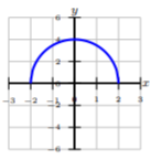
In the next example, we lightly discuss the idea of restricting the domain of a function. See, not all functions are one-to-one, i.e., not all functions’ graphs pass the horizontal line test. Could we make functions one-to-one? Could we force a graph of a function to pass the horizontal line test? Yes! This is where we restrict the domain of a function so that a piece of the function is one-to-one. Let’s take a simple function from the library, \(f(x) = x^{2}\). This function is not one-to-one:
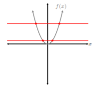
From the figure above, the graph of \(f(x) = x^{2}\) fails the horizontal line test. However, let’s restrict the domain of \(f(x)\) from \((−∞, ∞)\) to \([0, ∞)\):
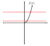
After graphing \(f(x) = x^{2}\) on the restricted domain \([0, ∞)\), we can see \(f(x)\) passes the horizontal line test, and, furthermore, is one-to-one. Careful! The function \(f(x) = x^{2}\) is only one-to-one on the restricted domain \([0, ∞)\).
Find and graph the inverse of \(f(x) = x^2\) on the restricted domain \([0, ∞)\).
Solution
Let’s first find the inverse function of \(f(x)\) on the restricted domain \([0, ∞)\).
\[\begin{aligned}f(x)&=x^2 \\ y&=x^2 \\ x&=y^2 \\ \pm\sqrt{x}&=y \\ f^{-1}(x)&=\sqrt{x}\end{aligned}\]
Notice, we omit the negative value of \(\sqrt{x}\) because we are on the restricted domain \([0, ∞)\), which doesn’t include negative values. Thus, the positive square root is the only solution on \([0, ∞)\). Next, we can graph \(f^{-1}(x)=\sqrt{x}\):
The graphs of \(f(x)\) and \(f^{−1} (x)\) are reflections of each other about the line \(y = x\):
Thus, the inverse function of of \(f(x) = x^2\) on the restricted domain \([0, ∞)\) is \(f^{−1} (x) =\sqrt{x}\).
Restricting the domain is a useful concept that used throughout mathematics. From inverse trigonometric functions to calculating integrals of functions with vertical asymptotes. Some of these concepts we discuss early in Algebra are critical in advanced mathematics.
Inverse Functions Homework
State whether the given relations are one-to-one.
\(\{(−2, 1),(−1, −1),(0, 3),(1, 1),(2, 3)\}\)
State whether the given functions are one-to-one. If not, state a restricted domain where the function can be one-to-one.
State whether the given functions are inverses by using the composition property.
\(\begin{aligned}g(x)&=-x^5 -3 \\ f(x)&=\sqrt[5]{-x-3}\end{aligned}\)
\(\begin{aligned}f(x)&=\dfrac{-x-1}{x-2} \\ g(x)&=\dfrac{-2x+1}{-x-1}\end{aligned}\)
\(\begin{aligned}g(x)&=-10x+5 \\ f(x)&=\dfrac{x-5}{10}\end{aligned}\)
\(\begin{aligned}f(x)&=-\dfrac{2}{x+3} \\ g(x)&=\dfrac{3x+2}{x+2}\end{aligned}\)
\(\begin{aligned}g(x)&=\sqrt[5]{\dfrac{x-1}{2}} \\ f(x)&=2x^5+1\end{aligned}\)
\(\begin{aligned}g(x)&=\dfrac{4-x}{x} \\ f(x)&=\dfrac{4}{x}\end{aligned}\)
\(\begin{aligned}h(x)&=\dfrac{-2-2x}{x} \\ f(x)&=\dfrac{-2}{x+2}\end{aligned}\)
\(\begin{aligned}f(x)&=\dfrac{x-5}{10} \\ h(x)&=10x+5\end{aligned}\)
\(\begin{aligned}f(x)&=\sqrt[5]{\dfrac{x+1}{2}} \\ g(x)&=2x^5-1\end{aligned}\)
\(\begin{aligned}g(x)&=\dfrac{8+9x}{2} \\ f(x)&=\dfrac{5x-9}{2}\end{aligned}\)
Find the inverse function of each one-to-one function.
\(f(x)=(x-2)^5+3\)
\(g(x)=\dfrac{4}{x+2}\)
\(f(x)=\dfrac{-2x-2}{x+2}\)
\(f(x)=\dfrac{10-x}{5}\)
\(g(x)=-(x-1)^3\)
\(f(x)=(x-3)^3\)
\(g(x)=\dfrac{x}{x-1}\)
\(f(x)=\dfrac{x-1}{x+1}\)
\(g(x)=\dfrac{8-5x}{4}\)
\(g(x)=-5x+1\)
\(g(x)=-1+x^3\)
\(h(x)=\dfrac{4-\sqrt[3]{4x}}{2}\)
\(f(x)=\dfrac{x+1}{x+2}\)
\(f(x)=\dfrac{7-3x}{x-2}\)
\(g(x)=-x\)
\(g(x)=\sqrt[3]{x+1}+2\)
\(f(x)=\dfrac{-3}{x-3}\)
\(g(x)=\dfrac{9+x}{3}\)
\(f(x)=\dfrac{5x-15}{2}\)
\(f(x)=\dfrac{12-3x}{4}\)
\(g(x)=\sqrt[5]{\dfrac{-x+2}{2}}\)
\(f(x)=\dfrac{-3-2x}{x+3}\)
\(h(x)=\dfrac{x}{x+2}\)
\(g(x)=\dfrac{-x+2}{3}\)
\(f(x)=\dfrac{5x-5}{4}\)
\(f(x)=3-2x^5\)
\(g(x)=(x-1)^3+2\)
\(f(x)=\dfrac{-1}{x+1}\)
\(f(x)=-\dfrac{3x}{4}\)
\(g(x)=\dfrac{-2x+1}{3}\)