3.1: Taylor’s Formula

Learning Objectives

• Explain the Taylor formula

As we saw in the previous chapter, representing functions as power series was a fruitful strategy for mathematicans in the eighteenth century (as it still is). Differentiating and integrating power series term by term was relatively easy, seemed to work, and led to many applications. Furthermore, power series representations for all of the elementary functions could be obtained if one was clever enough.

However, cleverness is an unreliable tool. Is there some systematic way to find a power series for a given function? To be sure, there were nagging questions: If we can find a power series, how do we know that the series we’ve created represents the function we started with? Even worse, is it possible for a function to have more than one power series representation centered at a given value \(a\)? This uniqueness issue is addressed by the following theorem.

Theorem \(\PageIndex{1}\)

If

\[f(x) = \sum_{n=0}^{\infty }a_n(x-a)^n\]

then

\[a_n = \frac{f^{(n)}(a)}{n!}\]

where \(f^{(n)}(a)\) represents the \(n^{th}\) derivative of \(f\) evaluated at \(a\).

A few comments about Theorem \(\PageIndex{1}\) are in order. Notice that we did not start with a function and derive its series representation. Instead we defined \(f(x)\) to be the series we wrote down. This assumes that the expression

\[\sum_{n=0}^{\infty }a_n(x-a)^n\]

actually has meaning (that it converges). At this point we have every reason to expect that it does, however expectation is not proof so we note that this is an assumption, not an established truth. Similarly, the idea that we can differentiate an infinite polynomial term-by-term as we would a finite polynomial is also assumed. As before, we follow in the footsteps of our \(18^{th}\) century forebears in making these assumptions. For now.

Exercise \(\PageIndex{1}\)

Prove Theorem \(\PageIndex{1}\).

Hint

\(f(a) = a_0 + a_1(a - a) + a_2(a - a)^2 +··· = a_0\), differentiate to obtain the other terms.

From Theorem \(\PageIndex{1}\) we see that if we do start with the function \(f(x)\) then no matter how we obtain its power series, the result will always be the same. The series

\[\sum_{n=0}^{\infty } \frac{f^{(n)}(a)}{n!} (x-a)^n = f(a) + f'(a)(x - a) + \frac{f''(a)}{2!}(x - a)^2 + \frac{f'''(a)}{3!}(x - a)^3 + \cdots \label{talyor}\]

is called the Taylor series for \(f\) expanded about (centered at) a. Although this systematic “machine” for obtaining power series for a function seems to have been known to a number of mathematicians in the early 1700’s, Brook Taylor was the first to publish this result in his Methodus Incrementorum (1715).

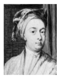
Figure \(\PageIndex{1}\): Brook Taylor.

The special case when \(a = 0\) was included by Colin Maclaurin in his Treatise of Fluxions (1742).

Thus when \(a = 0\), the series in Equation \ref{talyor} is simplified to

\[\sum_{n=0}^{\infty } \frac{f^{(n)}(0)}{n!} x^n \label{maclaurin} \]

and this series is often called the Maclaurin Series for \(f\).

The “prime notation” for the derivative was not used by Taylor, Maclaurin or their contemporaries. It was introduced by Joseph Louis Lagrange in his 1779 work Théorie des Fonctions Analytiques. In that work, Lagrange sought to get rid of Leibniz’s infinitesimals and base calculus on the power series idea. His idea was that by representing every function as a power series, calculus could be done “algebraically” by manipulating power series and examining various aspects of the series representation instead of appealing to the “controversial” notion of infinitesimals. He implicitly assumed that every continuous function could be replaced with its power series representation.

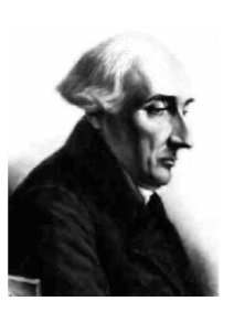
Figure \(\PageIndex{2}\): Joseph-Louis Lagrange.

That is, he wanted to think of the Taylor series as a “great big polynomial,” because polynomials are easy to work with. It was a very simple, yet exceedingly clever and far-reaching idea. Since \(e^x = 1 + x + x^2/2 + ...\), for example, why not just define the exponential to be the series and work with the series. After all, the series is just a very long polynomial.

This idea did not come out of nowhere. Leonhard Euler had put exactly that idea to work to solve many problems throughout the \(18^{th}\) century. Some of his solutions are still quite breath-taking when you first see them [14].

Taking his cue from the Taylor series \(\sum_{n=0}^{\infty } \frac{f^{(n)}(a)}{n!} (x - a)^n\) Lagrange observed that the coefficient of \((x - a)^n\) provides the derivative of \(f\) at \(a\) (divided by \(n!\)). Modifying the formula above to suit his purpose, Lagrange supposed that every differentiable function could be represented as

\[f(x) = \sum_{n=0}^{\infty } g_n(a) (x - a)^n\]

If we regard the parameter \(a\) as a variable then \(g_1\) is the derivative of \(f\), \(g_2 = 2f''\) and generally

\[g_n = n!f^{(n)}\]

Lagrange dubbed his function \(g_1\) the “fonction dérivée” from which we get the modern name “derivative.”

All in all, this was a very clever and insightful idea whose only real flaw is that its fundamental assumption is not true. It turns out that not every differentiable function can be represented as a Taylor series. This was demonstrated very dramatically by Augustin Cauchy’s famous counter-example

\[f(x) = \begin{cases} e^{-\frac{1}{x^2}} & \text{ if } x\neq 0 \\ 0 & \text{ if } x= 0 \end{cases}\]

This function is actually infinitely differentiable everywhere but its Maclaurin series (that is, a Taylor series with \(a = 0\)) does not converge to f because all of its derivatives at the origin are equal to zero: \(f^{(n)}(0) = 0,\forall n \in \mathbb{N}\)\)

Not every differentiable function can be represented as a Taylor series.

Computing these derivatives using the definition you learned in calculus is not conceptually difficult but the formulas involved do become complicated rather quickly. Some care must be taken to avoid error.

To begin with, let’s compute a few derivatives when \(x\neq 0\).

\[ \begin{align*} f^{(0)}(x) &= e^{x^{-2}} \\[4pt] f^{(1)}(x) &= 2x^{-3}e^{-x^{-2}} \\[4pt] f^{(2)}(x) &= (4x^{-6}-6x^{-4})e^{-x^{-2}} \end{align*}\]

As you can see the calculations are already getting a little complicated and we’ve only taken the second derivative. To streamline things a bit we take \(y = x - 1\), and define \(p_2(x) = 4x^6 - 6x^4\) so that

\[f^{(2)}(x) = p_2(x^{-1})e^{-x^{-2}} = p_2(y)e^{-y^{2}}\]

Exercise \(\PageIndex{2}\)

1. Adopting the notation \(y = x^{-1}\) and \(f^{(n)}(x) = p_n(y)e^{-y^{2}}\), find \(p_{n+1}(y)\) in terms of \(p_n(y)\). [Note: Don’t forget that you are differentiating with respect to \(x\), not \(y\).]
2. Use induction on n to show that \(p_n(y)\) is a polynomial for all \(n \in \mathbb{N}\).

Unfortunately everything we’ve done so far only gives us the derivatives we need when \(x\) is not zero, and we need the derivatives when \(x\) is zero. To find these we need to get back to very basic ideas.

Let’s assume for the moment that we know that \(f^{(n)}(0) = 0\) and recall that

\[f^{(n+1)}(0) = \lim_{x\to 0} \frac{f^{(n)}(x) - f^{(n)}(0)}{x-0}\]

\[f^{(n+1)}(0) = \lim_{x\to 0} x^{-1} p_n(x^{-1})e^{-x^{-2}}\]

\[f^{(n+1)}(0) = \lim_{y\to \pm \infty } \frac{yp_n(y)}{e^{y^{2}}}\]

We can close the deal with the following problem.

Exercise \(\PageIndex{3}\)

1. Let m be a nonnegative integer. Show that \(\lim_{y\to \pm \infty } \frac{y^m}{e^{y^{2}}} = 0\). [Hint: Induction and a dash of L’Hôpital’s rule should do the trick.]
2. Prove that \(\lim_{y\to \pm \infty } \frac{q(y)}{e^{y^{2}}} = 0\) for any polynomial \(q\).
3. Let \(f(x)\) be as in equation \(\PageIndex{4}\) and show that for every nonnegative integer \(n\), \(f^{(n)}(0) = 0\).

This example showed that while it was fruitful to exploit Taylor series representations of various functions, basing the foundations of calculus on power series was not a sound idea.

While Lagrange’s approach wasn’t totally successful, it was a major step away from infinitesimals and toward the modern approach. We still use aspects of it today. For instance we still use his prime notation (\(f'\)) to denote the derivative.

Turning Lagrange’s idea on its head it is clear that if we know how to compute derivatives, we can use this machine to obtain a power series when we are not “clever enough” to obtain the series in other (typically shorter) ways. For example, consider Newton’s binomial series when \(α = \frac{1}{2}\). Originally, we obtained this series by extending the binomial theorem to non-integer exponents.

Taylor’s formula provides a more systematic way to obtain this series:

\[f(x) = (1+x)^{\frac{1}{2}} ;\qquad f(0) = 1\]

\[f'(x) = \frac{1}{2}(1+x)^{\frac{1}{2}-1} ;\qquad f'(0) = \frac{1}{2}\]

\[f''(x) = \frac{1}{2}\left ( \frac{1}{2} - 1 \right )(1+x)^{\frac{1}{2}-2} ;\qquad f''(0) = \frac{1}{2}\left ( \frac{1}{2} - 1 \right )\]

and in general since

\[f^{(n)}(x) = \frac{1}{2}\left ( \frac{1}{2} - 1 \right )\cdots \frac{1}{2}\left ( \frac{1}{2} - (n - 1) \right )(1+x)^{\frac{1}{2}-n}\]

we have

\[f^{(n)}(0) = \frac{1}{2}\left ( \frac{1}{2} - 1 \right )\cdots \frac{1}{2}\left ( \frac{1}{2} - (n - 1) \right )\]

Using Taylor’s formula we obtain the series

\[\sum_{n=0}^{\infty }\frac{f^{(n)}(0)}{n!}x^n = 1 + \sum_{n=1}^{\infty }\frac{\frac{1}{2}\left ( \frac{1}{2} - 1 \right )\cdots \left ( \frac{1}{2} - (n - 1) \right )}{n!}x^n = 1 + \sum_{n=1}^{\infty }\frac{\prod_{j=0}^{n-1}\left ( \frac{1}{2}-j \right )}{n!}x^n\]

which agrees with equation 2.2.40 in the previous chapter.

Exercise \(\PageIndex{4}\)

Use Taylor’s formula to obtain the general binomial series \[(1+x)^{\alpha } = 1 + \sum_{n=1}^{\infty }\frac{\prod_{j=0}^{n-1}\left ( \alpha -j \right )}{n!}x^n\]

Exercise \(\PageIndex{5}\)

Use Taylor’s formula to obtain the Taylor series for the functions \(e^x\), \(\sin x\), and \(\cos x\) expanded about \(a\).

As you can see, Taylor’s “machine” will produce the power series for a function (if it has one), but is tedious to perform. We will find, generally, that this tediousness can be an obstacle to understanding. In many cases it will be better to be clever if we can. This is usually shorter. However, it is comforting to have Taylor’s formula available as a last resort.

The existence of a Taylor series is addressed (to some degree) by the following.

Theorem \(\PageIndex{2}\)

If \(f', f'', ..., f^{(n+1)}\) are all continuous on an interval containing \(a\) and \(x\), then

\[f(x) = f(a) + \frac{f'(a)}{1!}(x-a) + \frac{f''(a)}{2!}(x-a)^2 + \cdots + \frac{f^{(n)}(a)}{n!}(x-a)^n + \frac{1}{n!}\int_{t=a}^{x}f^{(n+1)}(t)(x-t)^ndt\]

Before we address the proof, notice that the \(n\)-th degree polynomial

\[f(a) + \frac{f'(a)}{1!}(x-a) + \frac{f''(a)}{2!}(x-a)^2 + \cdots + \frac{f^{(n)}(a)}{n!}(x-a)^n\]

resembles the Taylor series and, in fact, is called the \(n\)-th degree Taylor polynomial of \(f\) about \(a\). Theorem \(\PageIndex{2}\) says that a function can be written as the sum of this polynomial and a specific integral which we will analyze in the next chapter. We will get the proof started and leave the formal induction proof as an exercise.

Notice that the case when \(n = 0\) is really a restatement of the Fundamental Theorem of Calculus. Specifically, the FTC says \(\int_{t=a}^{x}f'(t)dt = f(x) - f(a)\) which we can rewrite as

\[f(x) = f(a) + \frac{1}{0!}\int_{t=a}^{x}f'(t)(x-t)^0dt\]

to provide the anchor step for our induction.

To derive the case where \(n = 1\), we use integration by parts. If we let

\[u = f'(t) \qquad dv = (x-t)^0dt\]

\[du = f''(t) \qquad v = -\frac{1}{1}(x-t)^1dt\]

we obtain

\[\begin{align*} f(x) &= f(a) + \frac{1}{0!}\left ( -\frac{1}{1}f'(t)(x-t)^1\mid _{t=a} ^x + \frac{1}{1}\int_{t=a}^{x}f''(t)(x-t)^1dt\right )\\ &= f(a) + \frac{1}{0!}\left ( -\frac{1}{1}f'(x)(x-x)^1+\frac{1}{1}f'(a)(x-a)^1 + \frac{1}{1}\int_{t=a}^{x}f''(t)(x-t)^1dt\right ) \\ &= f(a) + \frac{1}{1!}f'(a)(x-a)^1 + \frac{1}{1!}\int_{t=a}^{x}f''(t)(x-t)^1dt \end{align*}\]

Exercise \(\PageIndex{6}\)

Provide a formal induction proof for Theorem \(\PageIndex{2}\).