
5.11: Integral Definitions of Some Functions
- Page ID
- 21247
This page is a draft and is under active development.

By Theorem 2 in §10, \(\int f\) exists on \(I\) whenever the function \(f : E^{1} \rightarrow E\) is regulated on \(I,\) and \(E\) is complete. Hence whenever such an \(f\) is given, we can define a new function \(F\) by setting
\[F=\int_{a}^{x} f\]
on I for some \(a \in I.\) This is a convenient method of obtaining new continuous functions, differentiable on \(I-Q\) (\(Q\) countable). We shall now apply it to obtain new definitions of some functions previously defined in a rather strenuous step-by-step manner.
I. Logarithmic and Exponential Functions. From our former definitions, we proved that
\[\ln x=\int_{1}^{x} \frac{1}{t} d t, \quad x>0.\]
Now we want to treat this as a definition of logarithms. We start by setting
\[f(t)=\frac{1}{t}, \quad t \in E^{1}, t \neq 0,\]
and \(f(0)=0\).
Then \(f\) is continuous on \(I=(0,+\infty)\) and \(J=(-\infty, 0),\) so it has an exact primitive on \(I\) and \(J\) separately (not on \(E^{1}\)). Thus we can now define the log function on \(I\) by
\[\int_{1}^{x} \frac{1}{t} d t=\log x \text { (also written } \ln x ) \text { for } x>0.\]
By the very definition of an exact primitive, the log function is continuous and differentiable on \(I=(0,+\infty)\); its derivative on \(I\) is \(f\). Thus we again have the symbolic formula
\[(\log x)^{\prime}=\frac{1}{x}, \quad x>0.\]
If \(x<0,\) we can consider \(\log (-x).\) Then the chain rule (Theorem 3 of §1) yields
\[(\log (-x))^{\prime}=\frac{1}{x}. \quad \text { (Verify!)}\]
Hence
\[(\log |x|)^{\prime}=\frac{1}{x} \quad \text { for } x \neq 0.\]
Other properties of logarithms easily follow from (1). We summarize them now.
(i) \(\log 1=\int_{1}^{1} \frac{1}{t} d t=0\).
(ii) \(\log x<\log y\) whenever \(0<x<y\).
(iii) \(\lim _{x \rightarrow+\infty} \log x=+\infty\) and \(\lim _{x \rightarrow 0^{+}} \log x=-\infty\).
(iv) The range of log is all of \(E^{1}\).
(v) For any positive \(x, y \in E^{1}\),
\[\log (x y)=\log x+\log y \text { and } \log \left(\frac{x}{y}\right)=\log x-\log y.\]
(vi) \(\log a^{r}=r \cdot \log a, a>0, r \in N\).
(vii) \(\log e=1,\) where \(e=\lim _{n \rightarrow \infty}\left(1+\frac{1}{n}\right)^{n}\).
- Proof
-
(ii) By (2), \((\log x)^{\prime}>0\) on \(I=(0,+\infty),\) so \(\log x\) is increasing on \(I\).
(iii) By Theorem 5 in §10,
\[\lim _{x \rightarrow+\infty} \log x=\int_{1}^{\infty} \frac{1}{t} d t=+\infty\]
since
\[\sum_{n=1}^{\infty} \frac{1}{n}=+\infty \quad \text {(Chapter 4, §13, Example (b)).}\]
Hence, substituting \(y=1 / x,\) we obtain
\[\lim _{y \rightarrow 0^{+}} \log y=\lim _{x \rightarrow+\infty} \log \frac{1}{x}.\]
However, by Theorem 2 in §5 (substituting \(s=1 / t\)),
\[\log \frac{1}{x}=\int_{1}^{1 / x} \frac{1}{t} d t=-\int_{1}^{x} \frac{1}{s} d s=-\log x.\]
Thus
\[\lim _{y \rightarrow 0^{+}} \log y=\lim _{x \rightarrow+\infty} \log \frac{1}{x}=-\lim _{x \rightarrow+\infty} \log x=-\infty\]
as claimed. (We also proved that \(\log \frac{1}{x}=-\log x.\))
(iv) Assertion (iv) now follows by the Darboux property (as in Chapter 4, §9, Example (b)).
(v) With \(x, y\) fixed, we substitute \(t=x s\) in
\[\int_{1}^{x y} \frac{1}{t} d t=\log x y\]
and obtain
\[\begin{aligned} \log x y &=\int_{1}^{x y} \frac{1}{t} d t=\int_{1 / x}^{y} \frac{1}{s} d s \\ &=\int_{1 / x}^{1} \frac{1}{s} d s+\int_{1}^{y} \frac{1}{s} d s \\ &=-\log \frac{1}{x}+\log y \\ &=\log x+\log y. \end{aligned}\]
Replacing \(y\) by \(1 / y\) here, we have
\[\log \frac{x}{y}=\log x+\log \frac{1}{y}=\log x-\log y.\]
Thus (v) is proved, and (vi) follows by induction over \(r\).
(vii) By continuity,
\[\log e=\lim _{x \rightarrow e} \log x=\lim _{n \rightarrow \infty} \log \left(1+\frac{1}{n}\right)^{n}=\lim _{n \rightarrow \infty} \frac{\log (1+1 / n)}{1 / n},\]
where the last equality follows by (vi). Now, L'Hôpital's rule yields
\[\lim _{x \rightarrow 0} \frac{\log (1+x)}{x}=\lim _{x \rightarrow 0} \frac{1}{1+x}=1.\]
Letting \(x\) run over \(\frac{1}{n} \rightarrow 0,\) we get (vii). \(\quad \square\)
Note 1. Actually, (vi) holds for any \(r \in E^{1},\) with \(a^{r}\) as in Chapter 2, §§11-12. One uses the techniques from that section to prove it first for rational \(r,\) and then it follows for all real \(r\) by continuity. However, we prefer not to use this now.
Next, we define the exponential function ("exp") to be the inverse of the log function. This inverse function exists; it is continuous (even differentiable) and strictly increasing on its domain (by Theorem 3 of Chapter 4, §9 and Theorem 3 of Chapter 5, §2) since the log function has these properties. From \((\log x)^{\prime}=1 / x\) we get, as in 2,
\[(\exp x)^{\prime}=\exp x \quad \text {(cf. §2, Example (B)).}\]
The domain of the exponential is the range of its inverse, i.e., \(E^{1}\) (cf. Theorem 1(iv)). Thus \(\exp x\) is defined for all \(x \in E^{1}.\) The range of exp is the domain of log, i.e., \((0,+\infty).\) Hence exp \(x>0\) for all \(x \in E^{1}.\) Also, by definition,
\[\begin{aligned} \exp (\log x) &=x \text { for } x>0 \\ \exp 0 &=1 \text { (cf. Theorem } 1(\mathrm{i}) ), \text { and } \\ \exp r &=e^{r} \text { for } r \in N. \end{aligned}\]
Indeed, by Theorem 1(vi) and (vii), log \(e^{r}=r \cdot \log e=r.\) Hence (6) follows. If the definitions and rules of Chapter 2, §§11-12 are used, this proof even works for any \(r\) by Note 1. Thus our new definition of exp agrees with the old one.
Our next step is to give a new definition of \(a^{r},\) for any \(a, r \in E^{1}(a>0).\) We set
\[\begin{aligned} a^{r} &=\exp (r \cdot \log a) \text { or } \\ \log a^{r} &=r \cdot \log a \quad\left(r \in E^{1}\right). \end{aligned}\]
In case \(r \in N\), (8) becomes Theorem 1(vi). Thus for natural \(r,\) our new definition of \(a^{r}\) is consistent with the previous one. We also obtain, for \(a, b>0\),
\[(a b)^{r}=a^{r} b^{r} ; \quad a^{r s}=\left(a^{r}\right)^{s} ; \quad a^{r+s}=a^{r} a^{s} ; \quad\left(r, s \in E^{1}\right).\]
The proof is by taking logarithms. For example,
\[\begin{aligned} \log (a b)^{r} &=r \log a b=r(\log a+\log b)=r \cdot \log a+r \cdot \log b \\ &=\log a^{r}+\log b^{r}=\log \left(a^{r} b^{r}\right). \end{aligned}\]
Thus \((a b)^{r}=a^{r} b^{r}.\) Similar arguments can be given for the rest of (9) and other laws stated in Chapter 2, §§11-12.
We can now define the exponential to the base \(a(a>0)\) and its inverse, log \(_{a},\) as before (see the example in Chapter 4, §5 and Example (b) in Chapter 4, §9). The differentiability of the former is now immediate from (7), and the rest follows as before.
II. Trigonometric Functions. These shall now be defined in a precise analytic manner (not based on geometry).
We start with an integral definition of what is usually called the principal value of the arcsine function,
\[\arcsin x=\int_{0}^{x} \frac{1}{\sqrt{1-t^{2}}} d t.\]
We shall denote it by \(F(x)\) and set
\[f(x)=\frac{1}{\sqrt{1-x^{2}}} \text { on } I=(-1,1).\]
\((F=f=0\) on \(E^{1}-I\).) Thus by definition, \(F=\int f\) on \(I\).
Note that \(\int f\) exists and is exact on \(I\) since \(f\) is continuous on \(I.\) Thus
\[F^{\prime}(x)=f(x)=\frac{1}{\sqrt{1-x^{2}}}>0 \quad \text {for } x \in I,\]
and so \(F\) is strictly increasing on \(I\). Also, \(F(0)=\int_{0}^{0} f=0\).
We also define the number \(\pi\) by setting
\[\frac{\pi}{2}=2 \arcsin \sqrt{\frac{1}{2}}=2 F(c)=2 \int_{0}^{c} f, \quad c=\sqrt{\frac{1}{2}}.\]
Then we obtain the following theorem.
\(F\) has the limits
\[F\left(1^{-}\right)=\frac{\pi}{2} \text { and } F\left(-1^{+}\right)=-\frac{\pi}{2}.\]
Thus \(F\) becomes relatively continuous on \(\overline{I}=[-1,1]\) if one sets
\[F(1)=\frac{\pi}{2} \text { and } F(-1)=-\frac{\pi}{2},\]
i.e.,
\[\arcsin 1=\frac{\pi}{2} \text { and } \arcsin (-1)=-\frac{\pi}{2}.\]
- Proof
-
We have
\[F(x)=\int_{0}^{x} f=\int_{0}^{c} f+\int_{c}^{x} f, \quad c=\sqrt{\frac{1}{2}}.\]
By substituting \(s=\sqrt{1-t^{2}}\) in the last integral and setting, for brevity, \(y=\) \(\sqrt{1-x^{2}},\) we obtain
\[\int_{c}^{x} f=\int_{c}^{x} \frac{1}{\sqrt{1-t^{2}}} d t=\int_{y}^{c} \frac{1}{\sqrt{1-s^{2}}} d s=F(c)-F(y). \quad \text {(Verify!)}\]
Now as \(x \rightarrow 1^{-},\) we have \(y=\sqrt{1-x^{2}} \rightarrow 0,\) and hence \(F(y) \rightarrow F(0)=0\) (for \(F\) is continuous at 0). Thus
\[F\left(1^{-}\right)=\lim _{x \rightarrow 1^{-}} F(x)=\lim _{y \rightarrow 0}\left(\int_{0}^{c} f+\int_{y}^{c} f\right)=\int_{0}^{c} f+F(c)=2 \int_{0}^{c} f=\frac{\pi}{2}.\]
Similarly, one gets \(F\left(-1^{+}\right)=-\pi / 2. \quad \square\)
The function \(F\) as redefined in Theorem 2 will be denoted by \(F_{0}.\) It is a primitive of \(f\) on the closed interval \(\overline{I}\) (exact on \(I).\) Thus \(F_{0}(x)=\int_{0}^{x} f,\) \(-1 \leq x \leq 1,\) and we may now write
\[\frac{\pi}{2}=\int_{0}^{1} f \text { and } \pi=\int_{-1}^{0} f+\int_{0}^{1} f=\int_{-1}^{1} f.\]
Note 2. In classical analysis, the last integrals are regarded as so-called improper integrals, i.e., limits of integrals rather than integrals proper. In our theory, this is unnecessary since \(F_{0}\) is a genuine primitive of \(f\) on \(\overline{I}.\)
For each integer \(n\) (negatives included), we now define \(F_{n} : E^{1} \rightarrow E^{1}\) by
\[\begin{aligned} F_{n}(x) &=n \pi+(-1)^{n} F_{0}(x) \text { for } x \in \overline{I}=[-1,1] \\ F_{n} &=0 & \text { on }-\overline{I}. \end{aligned}\]
\(F_{n}\) is called the \(n\) th branch of the arcsine. Figure 26 shows the graphs of \(F_{0}\) and \(F_{1}\) ( that of \(F_{1}\) is dotted). We now obtain the following theorem.
(i) Each \(F_{n}\) is differentiable on \(I=(-1,1)\) and relatively continuous on \(\overline{I}=[-1,1]\).
(ii) \(F_{n}\) is increasing on \(\overline{I}\) if \(n\) is even, and decreasing if \(n\) is odd.
(iii) \(F_{n}^{\prime}(x)=\frac{(-1)^{n}}{\sqrt{1-x^{2}}}\) on \(I\).
(iv) \(F_{n}(-1)=F_{n-1}(-1)=n \pi-(-1)^{n} \frac{\pi}{2} ; F_{n}(1)=F_{n-1}(1)=n \pi+(-1)^{n} \frac{\pi}{2}\).
- Proof
-
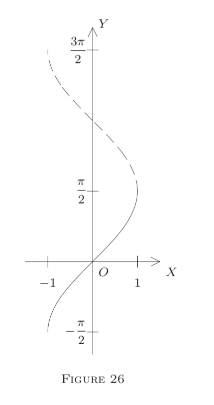
The proof is obvious from (12) and the properties of \(F_{0}.\) Assertion (iv) ensures that the graphs of the \(F_{n}\) add up to one curve. By (ii), each \(F_{n}\) is one to one (strictly monotone) on \(\overline{I} .\) Thus it has a strictly monotone inverse on the interval \(\overline{J_{n}}=F_{n}\) \([\![ -1, 1 ]\!] \), i.e., on the \(F_{n}\) -image of \(\overline{I}\). For simplicity, we consider only
\[\overline{J_{0}}=\left[-\frac{\pi}{2}, \frac{\pi}{2}\right] \text { and } J_{1}=\left[\frac{\pi}{2}, \frac{3 \pi}{2}\right],\]
as shown on the \(Y\) -axis in Figure 26. On these, we define for \(x \in \overline{J_{0}}\)
\[\sin x=F_{0}^{-1}(x)\]
and
\[\cos x=\sqrt{1-\sin ^{2} x},\]
and for \(x \in \overline{J_{1}}\)
\[\sin x=F_{1}^{-1}(x)\]
and
\[\cos x=-\sqrt{1-\sin ^{2} x}.\]
On the rest of \(E^{1},\) we define \(\sin x\) and \(\cos x\) periodically by setting
\[\sin (x+2 n \pi)=\sin x \text { and } \cos (x+2 n \pi)=\cos x, \quad n=0, \pm 1, \pm 2, \ldots.\]
Note that by Theorem 3(iv),
\[F_{0}^{-1}\left(\frac{\pi}{2}\right)=F_{1}^{-1}\left(\frac{\pi}{2}\right)=1.\]
Thus (13) and (14) both yield \(\sin \pi / 2=1\) for the common endpoint \(\pi / 2\) of \(\overline{J_{0}}\) and \(\overline{J_{1}},\) so the two formulas are consistent. We also have
\[\sin \left(-\frac{\pi}{2}\right)=\sin \left(\frac{3 \pi}{2}\right)=-1,\]
in agreement with (15). Thus the sine and cosine functions (briefly, \(s\) and \(c\)) are well defined on \(E^{1}\).
The sine and cosine functions (\(s\) and \(c\)) are differentiable, hence continuous, on all of \(E^{1},\) with derivatives \(s^{\prime}=c\) and \(c^{\prime}=-s;\) that is,
\[(\sin x)^{\prime}=\cos x \text { and }(\cos x)^{\prime}=-\sin x.\]
- Proof
-
It suffices to consider the intervals \(\overline{J_{0}}\) and \(\overline{J_{1}},\) for by (15), all properties of \(s\) and \(c\) repeat themselves, with period \(2 \pi,\) on the rest of \(E^{1}\).
By (13),
\[s=F_{0}^{-1} \text { on } \overline{J_{0}}=\left[-\frac{\pi}{2}, \frac{\pi}{2}\right],\]
where \(F_{0}\) is differentiable on \(I=(-1,1).\) Thus Theorem 3 of §2 shows that \(s\) is differentiable on \(J_{0}=(-\pi / 2, \pi / 2)\) and that
\[s^{\prime}(q)=\frac{1}{F_{0}^{\prime}(p)} \text { whenever } p \in I \text { and } q=F_{0}(p);\]
i.e., \(q \in J\) and \(p=s(q).\) However, by Theorem 3(iii),
\[F_{0}^{\prime}(p)=\frac{1}{\sqrt{1-p^{2}}}.\]
Hence,
\[s^{\prime}(q)=\sqrt{1-\sin ^{2} q}=\cos q=c(q), \quad q \in J.\]
This proves the theorem for interior points of \(\overline{J_{0}}\) as far as \(s\) is concerned.
As
\[c=\sqrt{1-s^{2}}=\left(1-s^{2}\right)^{\frac{1}{2}} \text{ on } J_{0} \text{ (by (13)),}\]
we can use the chain rule (Theorem 3 in §1) to obtain
\[c^{\prime}=\frac{1}{2}\left(1-s^{2}\right)^{-\frac{1}{2}}(-2 s) s^{\prime}=-s\]
on noting that \(s^{\prime}=c=\left(1-s^{2}\right)^{\frac{1}{2}}\) on \(J_{0}.\) Similarly, using (14), one proves that \(s^{\prime}=c\) and \(c^{\prime}=-s\) on \(J_{1}\) (interior of \(\overline{J_{1}})\).
Next, let \(q\) be an endpoint, say, \(q=\pi / 2.\) We take the left derivative
\[s_{-}^{\prime}(q)=\lim _{x \rightarrow q^{-}} \frac{s(x)-s(q)}{x-q}, \quad x \in J_{0}.\]
By L'Hôpital's rule, we get
\[s_{-}^{\prime}(q)=\lim _{x \rightarrow q^{-}} \frac{s^{\prime}(x)}{1}=\lim _{x \rightarrow q^{-}} c(x)\]
since \(s^{\prime}=c\) on \(J_{0}.\) However, \(s=F_{0}^{-1}\) is left continuous at \(q\) (why?); hence so is \(c=\sqrt{1-s^{2}}.\) (Why?) Therefore,
\[s_{-}^{\prime}(q)=\lim _{x \rightarrow q^{-}} c(x)=c(q), \quad \text {as required.}\]
Similarly, one shows that \(s_{+}^{\prime}(q)=c(q).\) Hence \(s^{\prime}(q)=c(q)\) and \(c^{\prime}(q)=-s(q)\) as before. \(\quad \square\)
The other trigonometric functions reduce to \(s\) and \(c\) by their defining formulas
\[\tan x=\frac{\sin x}{\cos x}, \cot x=\frac{\cos x}{\sin x}, \sec x=\frac{1}{\cos x}, \text { and } \csc x=\frac{1}{\sin x},\]
so we shall not dwell on them in detail. The various trigonometric laws easily follow from our present definitions; for hints, see the problems below.