1.8: Complex Functions as Mappings

A complex function \(w = f(z)\) is hard to graph because it takes 4 dimensions: 2 for \(z\) and 2 for \(w\). So, to visualize them we will think of complex functions as mappings. That is we will think of \(w = f(z)\) as taking a point in the complex \(z\)-plane and mapping (sending) it to a point in the complex \(w\)-plane.

We will use the following terms and symbols to discuss mappings.

• A function \(w = f(z)\) will also be called a mapping of \(z\) to \(w\).
• Alternatively we will write \(z \mapsto w\) or \(z \mapsto f(z)\). This is read as "\(z\) maps to \(w\)".
• We will say that "\(w\) is the image of \(z\) under the mapping" or more simply "\(w\) is the image of \(z\)".
• If we have a set of points in the \(z\)-plane we will talk of the image of that set under the mapping.
  For example, under the mapping \(z \mapsto iz\) the image of the imaginary \(z\)-axis is the real \(w\)-axis.

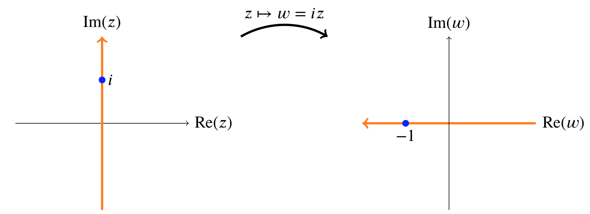
The image of the imaginary axis under \(z \mapsto iz\)

Example \(\PageIndex{1}\)

The mapping \(w = z^2\). We visualize this by putting the \(z\)-plane on the left and the \(w\)-plane on the right. We then draw various curves and regions in the \(z\)-plane and the corresponding image under \(z^2\) in the \(w\)-plane.

In the first figure we show that rays from the origin are mapped by \(z^2\) to rays from the origin. We see that

1. The ray \(L_2\) at \(\pi /4\) radians is mapped to the ray \(f(L_2)\) at \(\pi /2\) radians.
2. The rays \(L_2\) and \(L_6\) are both mapped to the same ray. This is true for each pair of diametrically opposed rays.
3. A ray at angle \(\theta\) is mapped to the ray at angle \(2 \theta\).

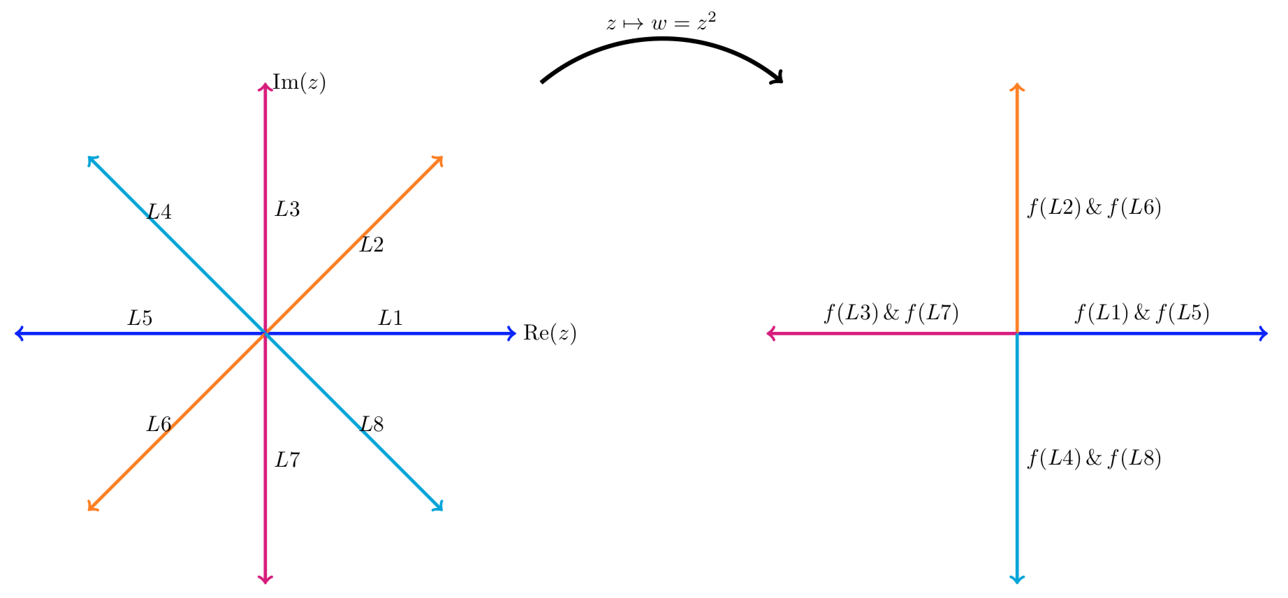
\(f(z) = z^2\) maps rays from the origin to rays from the origin.

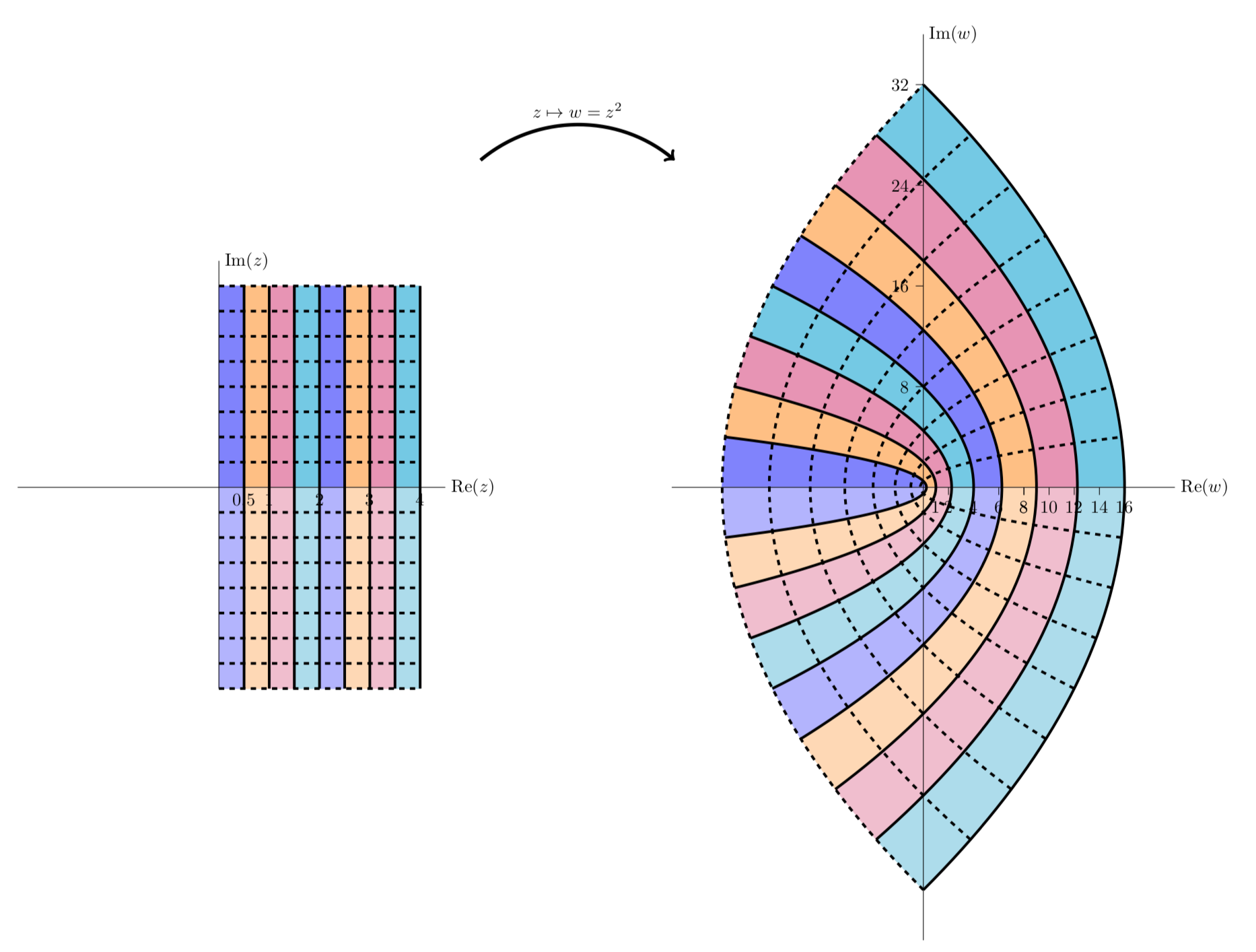
The next figure gives another view of the mapping. Here we see vertical stripes in the first quadrant are mapped to parabolic stripes that live in the first and second quadrants.

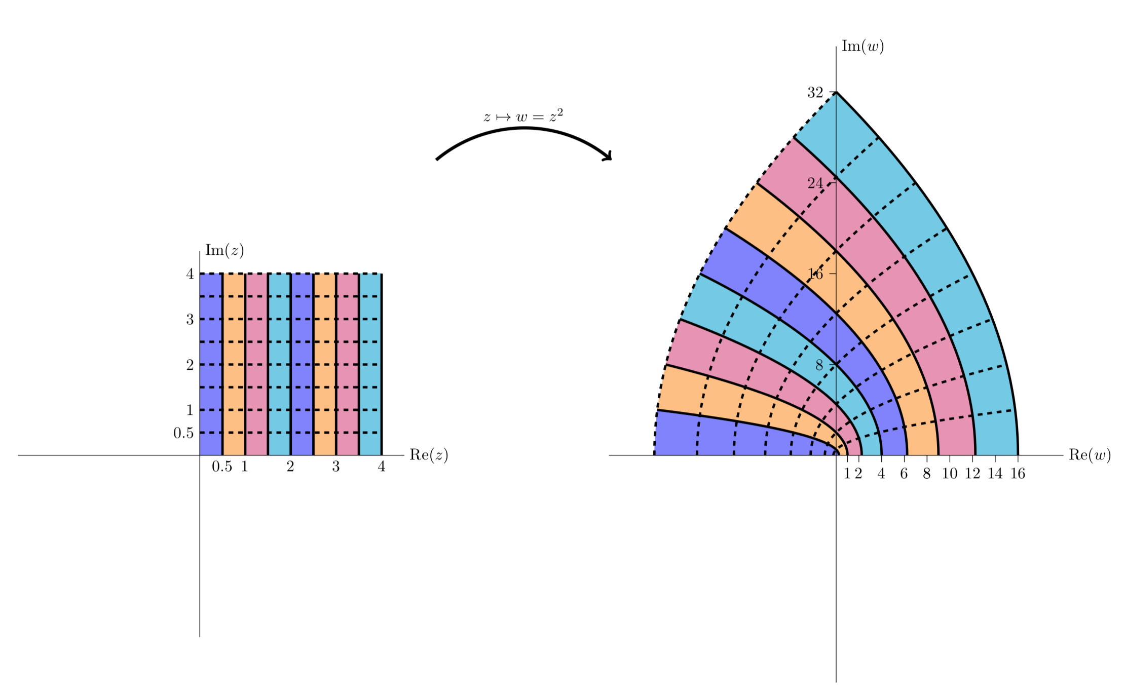
\(z^2 = (x^2 - y^2) + i2xy\) maps vertical lines to left facing parabolas.

The next figure is similar to the previous one, except in this figure we look at vertical stripes in both the first and second quadrants. We see that they map to parabolic stripes that live in all four quadrants.

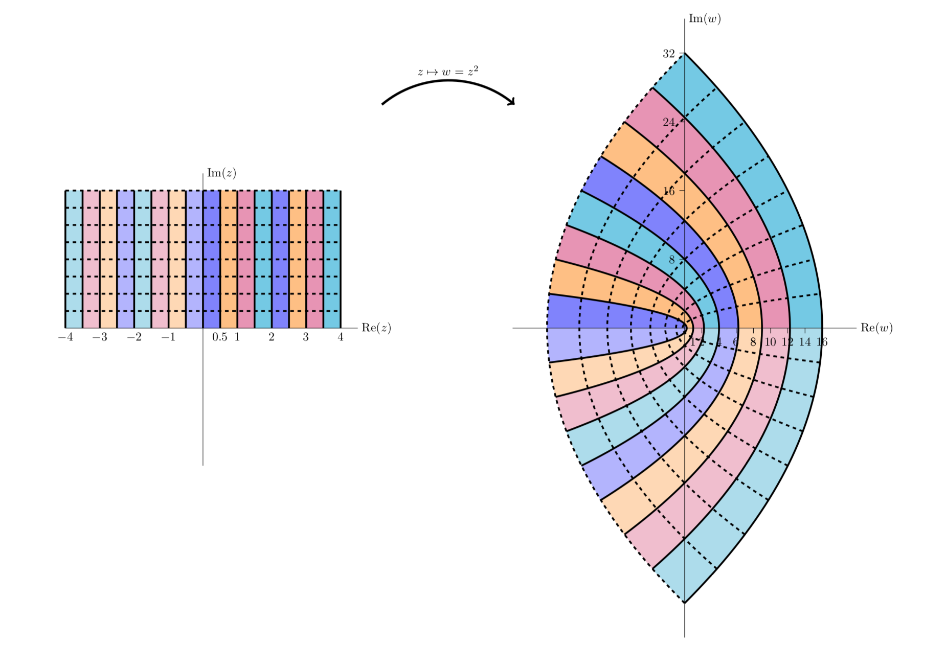
\(f(z) = z^2\) maps the first two quadrants to the entire plane.

The next figure shows the mapping of stripes in the first and fourth quadrants. The image map is identical to the previous figure. This is because the fourth quadrant is minus the second quadrant, but \(z^2 = (-z)^2\)

Vertical stripes in quadrant 4 are mapped identically to vertical stripes in quadrant 2.

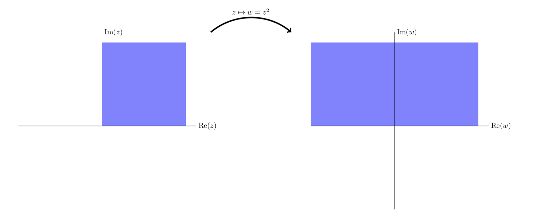
Simplified view of the first quadrant being mapped to the first two quadrants.

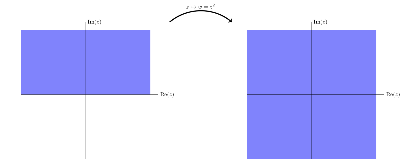
Simplified view of the first two quadrants being mapped to the entire plane.

Example \(\PageIndex{2}\)

The mapping \(w = e^z\). Here we present a series of plots showing how the exponential function maps \(z\) to \(w\).

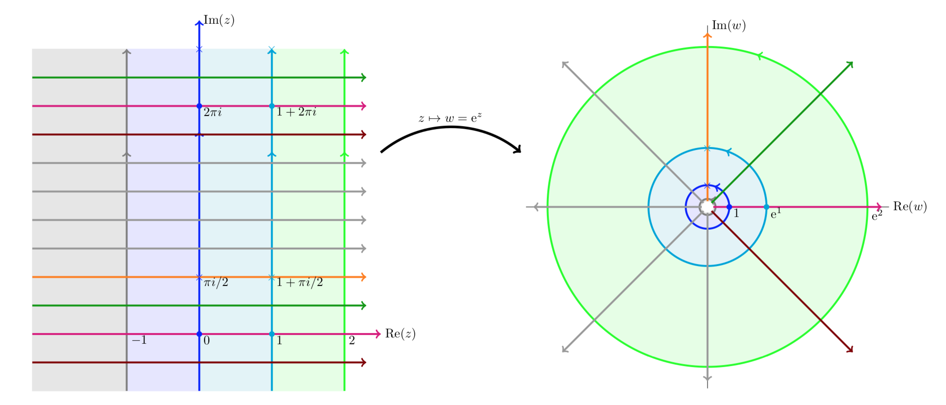
Notice that vertical lines are mapped to circles and horizontal lines to rays from the origin.

The next four figures all show essentially the same thing: the exponential function maps horizontal stripes to circular sectors. Any horizontal stripe of width \(2\pi\) gets mapped to the entire plane minus the origin,

Because the plane minus the origin comes up frequently we give it a name:

Definition: punctured plane

The punctured plane is the complex plane minus the origin. In symbols we can write it as \(C\) - {0} or \(C\)/{0}.

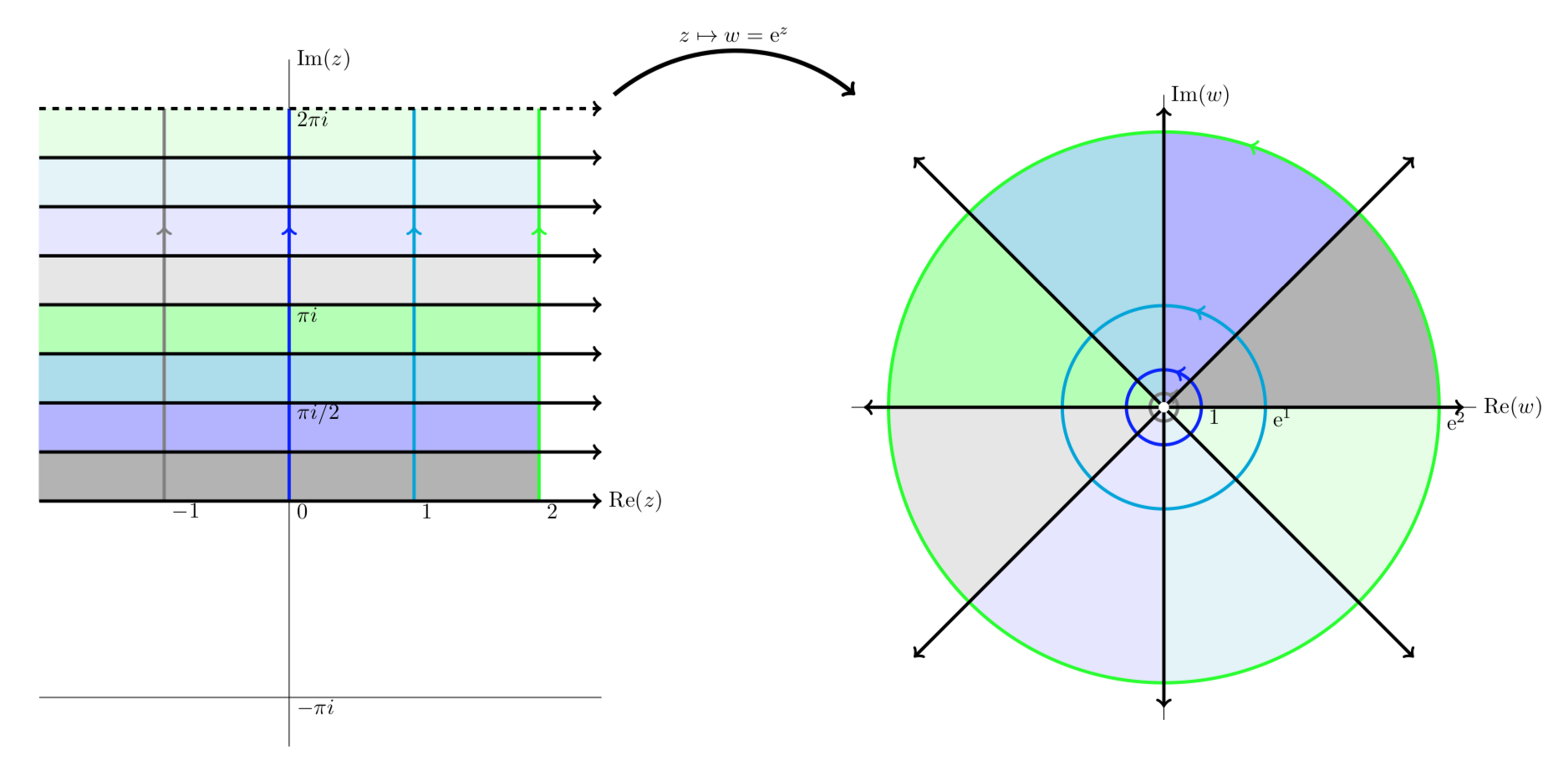
The horizontal strip \(0 \le y < 2\pi\) is mapped to the punctured plane

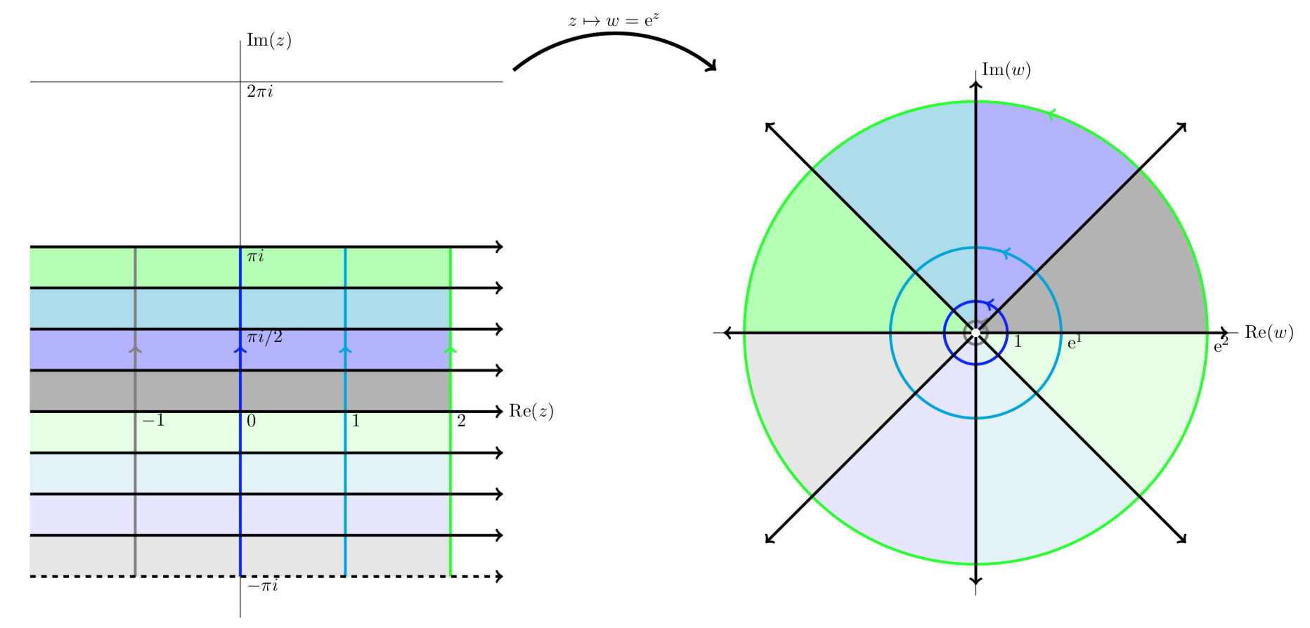
The horizontal strip \(-\pi < y \le \pi\) is mapped to the punctured plane

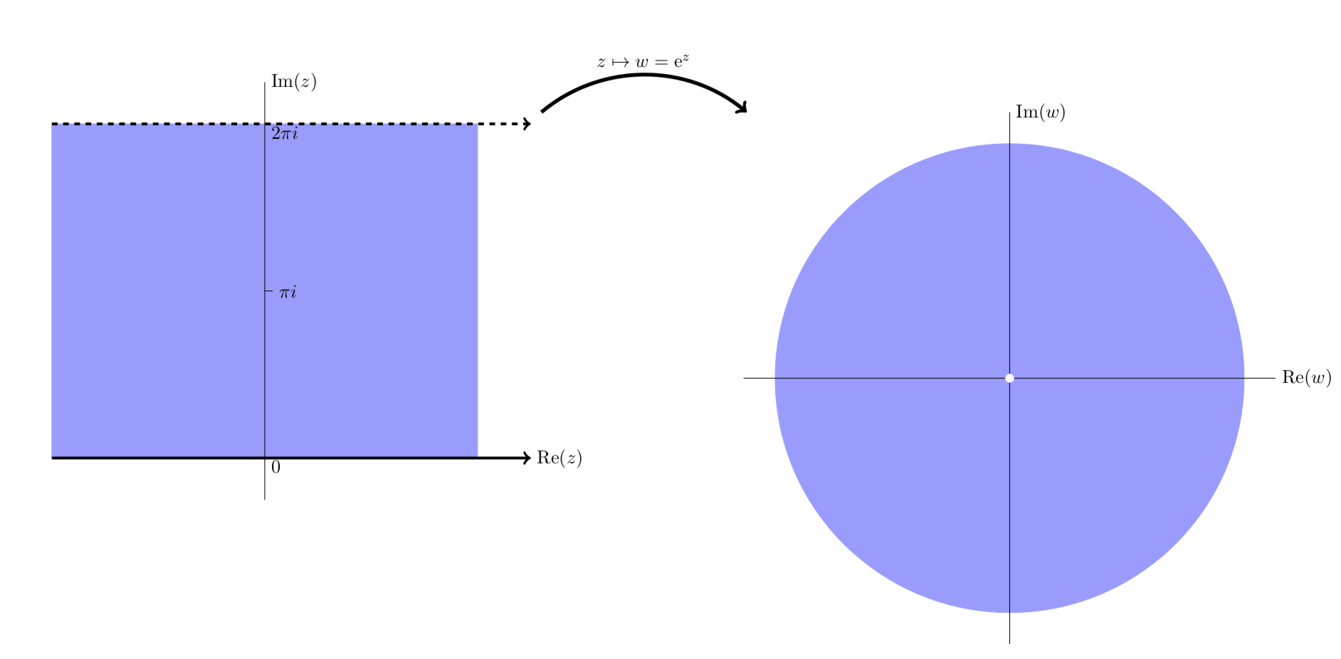
Simplified view showing \(e^z\) maps the horizontal stripe \(0 \le y < 2\pi\) to the punctured plane.

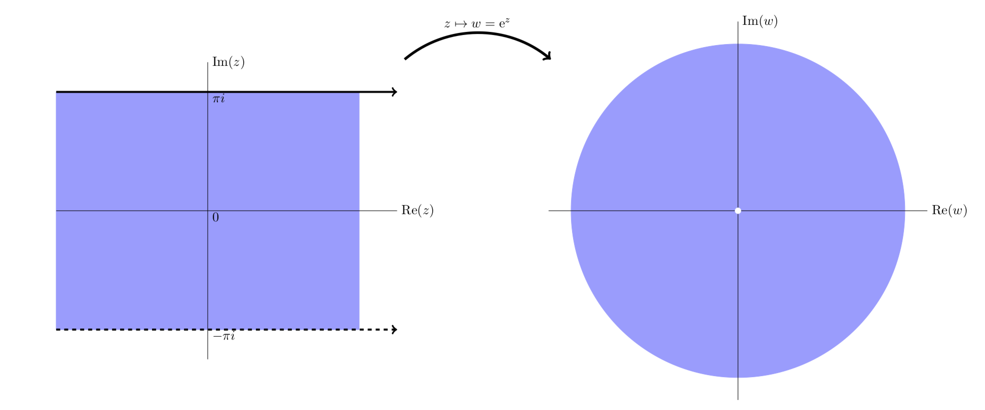
Simplified view showing \(e^z\) maps the horizontal stripe \(-\pi < y \le \pi\) to the punctured plane.