
11.9: Flows around cylinders
- Page ID
- 51145

Milne-Thomson circle theorem
The Milne-Thomson theorem allows us to insert a circle into a two-dimensional flow and see how the flow adjusts. First we’ll state and prove the theorem.
If \(f(z)\) is a complex potential with all its singularities outside \(|z| = R\) then
\[\Phi (z) = f(z) + \overline{f(\dfrac{R^2}{\overline{z}})} \nonumber \]
is a complex potential with streamline on \(|z| = R\) and the same singularities as \(f\) in the region \(|z| > R\).
- Proof
-
First note that \(R^2/\overline{z}\) is the reflection of \(z\) in the circle \(|z| = R\).
Next we need to see that \(\overline{f(R^2/\overline{z})}\) is analytic for \(|z| > R\). By assumption \(f(z)\) is analytic for \(|z| < R\), so it can be expressed as a Taylor series
\[f(z) = a_0 + a_1 z + a_2 z^2 + \ ... \nonumber \]
Therefore,
\[\overline{f(\dfrac{R^2}{\overline{z}})} = \overline{a_0} + \overline{a_1} \dfrac{R^2}{z} + \overline{a_2} (\dfrac{R^2}{z})^2 + \ ... \nonumber \]
All the singularities of \(f\) are outside \(|z| = R\), so the Taylor series in Equation 11.10.2 converges for \(|z| \le R\). This means the Laurent series in Equation 11.10.3 converges for \(|z| \ge R\). That is, \(\overline{f(R^2/\overline{z})}\) is analytic \(|z| \ge R\), i.e. it introduces no singularies to \(\Phi (z)\) outside \(|z| = R\).
The last thing to show is that \(|z| = R\) is a streamline for \(\Phi (z)\). This follows because for \(z = Re^{i \theta}\)
\[\Phi (Re^{i \theta}) = f(Re^{i \theta} + \overline{f(Re^{i \theta})} \nonumber \]
is real. Therefore
\[\psi (Re^{i \theta} = \text{Im} (\Phi (Re^{i \theta}) = 0. \nonumber \]
Examples
Think of \(f(z)\) as representing flow, possibly with sources or vortices outside \(|z| = R\). Then \(\Phi (z)\) represents the new flow when a circular obstacle is placed in the flow. Here are a few examples.
We know from Topic 6 that \(f(z) = z\) is the complex potential for uniform flow to the right. So,
\[\Phi (z) = z + R^2/z \nonumber \]
is the potential for uniform flow around a circle of radius \(R\) centered at the origin.
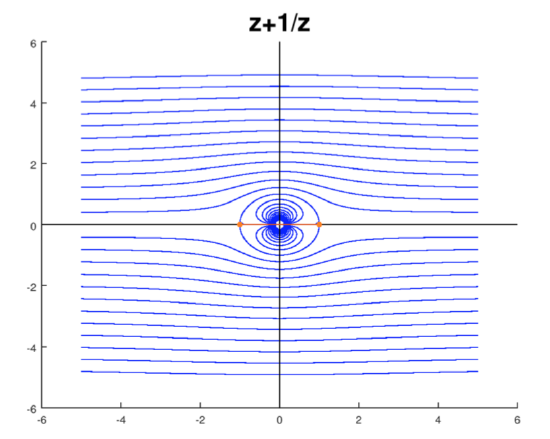
Uniform flow around a circle
Just because they look nice, the figure includes streamlines inside the circle. These don’t interact with the flow outside the circle.
Note, that as \(z\) gets large flow looks uniform. We can see this analytically because
\[\Phi '(z) = 1 - R^2/z^2 \nonumber \]
goes to 1 as \(z\) gets large. (Recall that the velocity field is (\(\phi _x, \phi _y\)), where \(\Phi = \phi + i \psi \ ...\))
Here the source is at \(z = -2\) (outside the unit circle) with complex potential
\[f(z) = \log (z + 2). \nonumber \]
With the appropriate branch cut the singularities of \(f\) are also outside \(|z| = 1\). So we can apply Milne-Thomson and obtain
\[\Phi (z) = \log (z + 2) + \overline{\log (\dfrac{1}{\overline{z}} + 2)} \nonumber \]
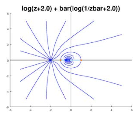
Source flow around a circle
We know that far from the origin the flow should look the same as a flow with just a source at \(z = -2\).
Let’s see this analytically. First we state a useful fact:
If \(g(z)\) is analytic then so is \(h(z) = \overline{g(\overline{z})}\) and \(h'(z) = \overline{g'(\overline{z})}\).
- Proof
-
Use the Taylor series for \(g\) to get the Taylor series for \(h\) and then compare \(h'(z)\) and \(\overline{g'(\overline{z})}\).
Using this we have
\[\Phi ' (z) = \dfrac{1}{z + 2} - \dfrac{1}{z(1 + 2z)} \nonumber \]
For large \(z\) the second term decays much faster than the first, so
\[\Phi ' (z) \approx \dfrac{1}{z + 2}. \nonumber \]
That is, far from \(z = 0\), the velocity field looks just like the velocity field for \(f(z)\), i.e. the velocity field of a source at \(z = -2\).
If we use
\[g(z) = z^2 \nonumber \]
we can transform a flow from the upper half-plane to the first quadrant
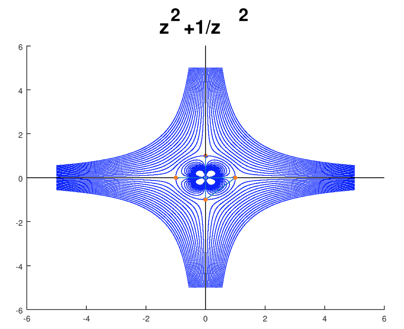
Source flow around a quarter circular corner