7.3: C- Differential Forms and Stokes' Theorem

Differential forms come up quite a bit in this book, especially in Chapter 4 and Chapter 5. Let us overview their definition and state the general Stokes’ theorem. No proofs are given, this appendix is just a bare bones guide. For a more complete introduction to differential forms, see Rudin [R2].

The short story about differential forms is that a \(k\)-form is an object that can be integrated (summed) over a \(k\)-dimensional object, taking orientation into account. For simplicity, as in most of this book, everything in this appendix is stated for smooth (\(C^\infty\)) objects to avoid worrying about how much regularity is needed.

The main point of differential forms is to find the proper context for the Fundamental Theorem of Calculus, \[\int_a^b f'(x) \, dx = f(b)-f(a) .\] We interpret both sides as integration. The left-hand side is an integral of the \(1\)-form \(f'\, dx\) over the \(1\)-dimensional interval \([a,b]\) and the right-hand side is an integral of the \(0\)-form, that is a function, \(f\) over the \(0\)-dimensional (two-point) set \(\{ a, b \}\). Both sides consider orientation, \([a,b]\) is integrated from \(a\) to \(b\), \(\{a\}\) is oriented negatively and \(\{b\}\) is oriented positively. The two-point set \(\{a,b\}\) is the boundary of \([a,b]\), and the orientation of \(\{ a,b \}\) is induced by \([a,b]\).

Let us define the objects over which we integrate, that is, smooth submanifolds of \(\mathbb{R}^n\). Our model for a \(k\)-dimensional submanifold-with-boundary is the upper-half-space and its boundary: \[\mathbb{H}^k \overset{\text{def}}{=} \{ x \in \mathbb{R}^k : x_k \geq 0 \} , \qquad \partial \mathbb{H}^k \overset{\text{def}}{=} \{ x \in \mathbb{R}^k : x_k = 0 \} ,\]

Definition: Embedded Submanifold-with-Boundary

Let \(M \subset \mathbb{R}^n\) have the induced subspace topology. Let \(k \in \mathbb{N}_0\). Let \(M\) have the property that for each \(p \in M\), there exists a neighborhood \(W \subset \mathbb{R}^n\) of \(p\), a point \(q \in \mathbb{H}^k\), a neighborhood \(U \subset \mathbb{H}^k\) of \(q\), and a smooth one-to-one open\(^{1}\) mapping \(\varphi \colon U \to M\) such that \(\varphi(q) = p\), the derivative \(D\varphi\) has rank \(k\) at all points, and \(\varphi(U) = M \cap W\). Then \(M\) is an embedded submanifold-with-boundary of dimension \(k\). The map \(\varphi\) is called a local parametrization. If \(q\) is such that \(q_k = 0\) (the last component is zero), then \(p = \varphi(q)\) is a boundary point. Let \(\partial M\) denote the set of boundary points. If \(\partial M = \emptyset\), then we say \(M\) is simply an embedded submanifold.

The situation for a boundary point and an interior point is depicted in Figure \(\PageIndex{1}\). Note that \(W\) is a bigger neighborhood in \(\mathbb{R}^n\) than the image \(\varphi(U)\).

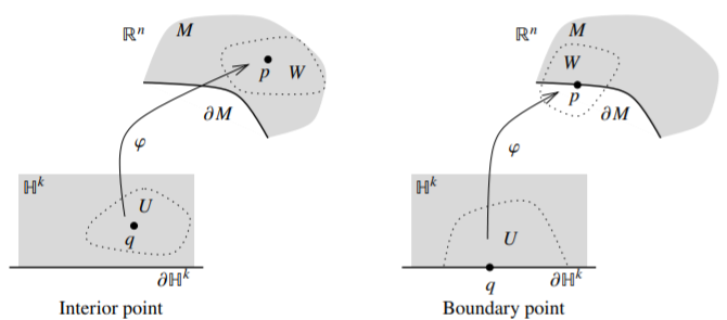
Figure \(\PageIndex{1}\)

Completely correctly, we should say submanifold of \(\mathbb{R}^{k}\). Sometimes people (including me) say manifold when they mean submanifold. A manifold is a more abstract concept, but all submanifolds are manifolds. The word embedded has to do with the topology on \(M\), and this has to do with the condition \(\varphi(U) = M \cap W\) and \(\varphi\) being open. The condition means that \(\varphi\) is a homeomorphism onto \(M \cap W\). It is important that \(W\) is an open set in \(\mathbb{R}^n\). For our purposes here, all submanifolds will be embedded. We have also made some economy in the definition. If \(q\) is not on the boundary of \(\mathbb{H}^k\), then we might as well have used \(\mathbb{R}^k\) instead of \(\mathbb{H}^k\). A submanifold is something that is locally like \(\mathbb{R}^k\), and if it has a boundary, then near the boundary it is locally like \(\mathbb{H}^k\) near a point of \(\partial \mathbb{H}^k\).

We also remark that submanifolds are often defined in reverse rather than by parametrizations, that is, by starting with the (relatively) open sets \(M \cap W\), and the maps \(\varphi^{-1}\), calling those charts, and calling the entire set of charts an atlas. The particular version of the definition we have chosen makes it easy to evaluate integrals in the same way that parametrizing curves makes it easy to evaluate integrals.

Examples of such submanifolds are domains with smooth boundaries as in Definition for Hypersurface, we can take the inclusion map \(x \mapsto x\) as our parametrization. The domain is then the submanifold \(M\) and \(\partial M\) is the boundary of the domain. Domains are the key application for our purposes. Another example are smooth curves.

If \(M\) is an embedded submanifold-with-boundary of dimension \(k\), then \(\partial M\) is also an embedded submanifold of dimension \(k-1\). Simply restrict the parametrizations to the boundary of \(\mathbb{H}^k\).

We also need to define an orientation.

Definition: Transition Map

Let \(M \subset \mathbb{R}^n\) be an embedded submanifold-with-boundary of dimension \(k \geq 2\). Suppose a set of parametrizations can be chosen such that each point of \(M\) is in the image of one of the parametrizations, and if \(\varphi \colon U \to M\) and \(\widetilde{\varphi} \colon \widetilde{U} \to M\) are two parametrizations such that \(\varphi(U) \cap \widetilde{\varphi}(\widetilde{U}) \not= \emptyset\), then the transition map (automatically smooth) defined by \[{\widetilde{\varphi}}^{~{-1}} \circ \varphi\] on \(\varphi^{-1}\bigl(\varphi(U) \cap \widetilde{\varphi}(\widetilde{U})\bigr)\) (in other words, wherever it makes sense) is orientation preserving, that is \[\det D\bigl({\widetilde{\varphi}}^{~{-1}} \circ \varphi \bigr) > 0\] at all points. The set of such parametrizations is the orientation on \(M\), and we usually take the maximal set of such parametrizations.

If \(M\) is oriented, then the restrictions of the parametrizations to \(\partial \mathbb{H}^k\) give an orientation on \(\partial M\). We say this is the induced orientation on \(\partial M\).

For dimensions \(k=0\) (isolated points) and \(k=1\) (curves) we must define orientation differently. For \(k=0\), we simply give each point an orientation of \(+\) or \(-\). For \(k=1\), we need to allow parametrization by open subsets not only of \(\mathbb{H}^1 = [0,\infty)\), but also \(-\mathbb{H}^1 = (-\infty,0]\). The definition is the same otherwise. To define the orientation of the boundary, if the boundary point corresponds to the \(0\) in \([0,\infty)\) we give this boundary point the orientation \(-\), and if it corresponds to the \(0\) in \((-\infty,0]\), then we give this point the orientation \(+\). The reason for this complication is that unlike in \(\mathbb{R}^k\) for \(k \geq 2\), the set \(\mathbb{H}^1 = [0,\infty)\) cannot be “rotated” (in \(\mathbb{R}^1\)) or mapped via an orientation preserving map onto \(-\mathbb{H}^1 = (-\infty,0]\), but in \(\mathbb{R}^2\) the upper-half-plane \(\mathbb{H}^2\) can be rotated to the lower-half-plane \(-\mathbb{H}^2 = \{ x \in \mathbb{R}^2 : x_2 \leq 0 \}\). For computations, it is often useful for compact curves with endpoints (boundary) to just give one parametrization from \([0,1]\) or perhaps \([a,b]\), then \(a\) corresponds to the \(-\) and \(b\) corresponds to the \(+\).

The fact that the transition map is smooth does require a proof, which is a good exercise in basic analysis. It requires a bit of care at boundary points.

An orientation allows us to have a well-defined integral on \(M\), just like a curve needs to be oriented in order to define a line integral. However, unlike for curves, not every submanifold of dimension more than one is orientable, that is, admits an orientation. A classical nonorientable example is the Möbius strip.

Now that we know “on” what we integrate, let us figure out what “it” is that we integrate. Let us start with \(0\)-forms. We define \(0\)-forms as smooth functions (possibly complex-valued). Sometimes we need a function defined just on a submanifold. A function \(f\) defined on a submanifold \(M\) is smooth when \(f \circ \varphi\) is smooth on \(U\) for every parametrization \(\varphi \colon U \to M\). Equivalently, one can prove that \(f\) is the restriction of some smooth function defined on some neighborhood of \(M\) in \(\mathbb{R}^n\).

A \(0\)-form \(\omega\) defined on a \(0\)-dimensional oriented submanifold \(M\) is integrated as \[\int_M \omega \overset{\text{def}}{=} \sum_{p \in M} \epsilon_p \omega(p) ,\] where \(\epsilon_p\) is the orientation of \(p\) given as \(+1\) or \(-1\). To avoid problems of integrability, one can assume that \(\omega\) is compactly supported (it is nonzero on at most finitely many points of \(M\)) or that \(M\) is compact (it is a finite set).

The correct definition of a \(1\)-form is that it is a “smooth section” of the dual of the vector bundle \(T \mathbb{R}^n\). That is, it is something that eats a vector field, and spits out a function. The \(1\)-form \(dx_k\) is supposed to be the object that does \[dx_k\left( \frac{\partial}{\partial x_k} \right) = 1, \qquad dx_k\left( \frac{\partial}{\partial x_j} \right) = 0 \quad \text{if $j\not=k$}.\] For our purposes here, just suppose that a \(1\)-form in \(\mathbb{R}^n\) is an object of the form \[\omega = g_1 dx_1 + g_2 dx_2 + \cdots + g_n dx_n ,\] where \(g_1, g_2, \ldots, g_n\) are smooth functions. That is, a \(1\)-form is at each point a linear combination of \(dx_1, dx_2, \ldots, dx_n\) that varies smoothly from point to point. Suppose \(M\) is a one-dimensional submanifold (possibly with boundary), \(\varphi \colon U \to M\) is a parametrization compatible with the orientation of \(M\), and \(g_j\) is supported in \(\varphi(U)\). Define \[\int_M \omega \overset{\text{def}}{=} \sum_{j=1}^n \int_U g_j\bigl( \varphi(t) \bigr) \varphi_j'(t) \, dt ,\] where the integral \(\int_U \cdots \, dt\) is evaluated with the usual positive orientation (left to right) as \(U \subset \mathbb{R}\), and \(\varphi_j\) is the \(j\)th component of \(\varphi\).

Generally, a \(1\)-form has support bigger than just \(\varphi(U)\). In this case, one needs to use a so-called partition of unity to write \(\omega\) as a locally finite sum \[\omega = \sum_{\ell} \omega_\ell ,\] where each \(\omega_\ell\) has support in the image of a single parametrization. By locally finite, we mean that on each compact neighborhood only finitely many \(\omega_\ell\) are nonzero. Define \[\int_M \omega \overset{\text{def}}{=} \sum_{\ell} \int_M \omega_\ell .\] The definition makes sense only if this sum actually exists. For example, if \(\omega\) is compactly supported, then this sum is only finite, and so it exists.

Higher degree forms are constructed out of \(1\)-forms and \(0\)-forms by the so-called wedge product. Given a \(k\)-form \(\omega\) and an \(\ell\)-form \(\eta\), \[\omega \wedge \eta\] is a \((k+\ell)\)-form. We require the wedge product to be bilinear at each point: If \(f\) and \(g\) are smooth functions, then \[(f \omega + g \eta) \wedge \xi = f (\omega \wedge \xi) + g (\eta \wedge \xi) , \qquad \text{and} \qquad \omega \wedge (f \eta + g \xi) = f (\omega \wedge \eta ) + g ( \omega \wedge \xi) .\] The wedge product is not commutative; we require it to be anticommutative on \(1\)-forms. If \(\omega\) and \(\eta\) are \(1\)-forms, then \[\omega \wedge \eta = - \eta \wedge \omega .\] The negative keeps track of orientation. When \(\omega\) is a \(k\)-form and \(\eta\) is an \(\ell\)-form, \[\omega \wedge \eta = {(-1)}^{k\ell} \eta \wedge \omega .\]

We wedge together the basis \(1\)-forms to get all \(k\)-forms. A \(k\)-form is then an expression \[\omega = \sum_{j_1=1}^n \sum_{j_2=1}^n \cdots \sum_{j_k=1}^n g_{j_1,\ldots,j_k} \, dx_{j_1} \wedge dx_{j_2} \wedge \cdots \wedge dx_{j_k} ,\] where \(g_{j_1,\ldots,j_k}\) are smooth functions. We can simplify even more. Since the wedge is anticommutative on \(1\)-forms, \[dx_j \wedge dx_m = -dx_m \wedge dx_j , \qquad \text{and} \qquad dx_j \wedge dx_j = 0 .\] In other words, every form \(dx_{j_1} \wedge dx_{j_2} \wedge \cdots \wedge dx_{j_k}\) is either zero, if any two indices from \(j_1,\ldots,j_k\) are equal, or can be put into the form \(\pm dx_{j_1} \wedge dx_{j_2} \wedge \cdots \wedge dx_{j_k}\), where \(j_1 < j_2 < \cdots < j_k\). Thus, a \(k\)-form can always be written as \[\omega = \sum_{1 \leq j_1 < j_2 < \cdots < j_k \leq n} g_{j_1,\ldots,j_k} \, dx_{j_1} \wedge dx_{j_2} \wedge \cdots \wedge dx_{j_k} .\]

Consider an oriented \(k\)-dimensional submanifold \(M\) (possibly with boundary), a parametrization \(\varphi \colon U \to M\) from the orientation, and a \(k\)-form \(\omega\) supported in \(\varphi(U)\) (that is each \(g_{j_1,\ldots,j_k}\) is supported in \(\varphi(U)\)). Denote by \(t \in U \subset \mathbb{R}^k\) the coordinates on \(U\). Define \[\int_M \omega \overset{\text{def}}{=} \sum_{1 \leq j_1 < j_2 < \cdots < j_k \leq n} \int_U g_{j_1,\ldots,j_k}(t) \det D (\varphi_{j_1},\varphi_{j_2},\ldots,\varphi_{j_k}) \, dt\] where the integral \(\int_U \cdots\, dt\) is evaluated in the usual orientation on \(\mathbb{R}^k\) with \(dt\) the standard measure on \(\mathbb{R}^k\) (think \(dt = dt_1 dt_2 \cdots dt_n\)), and \(D (\varphi_{j_1},\varphi_{j_2},\ldots,\varphi_{j_k})\) denotes the derivative of the mapping whose \(\ell\)th component is \(\varphi_{j_\ell}\).

Similarly as before, if \(\omega\) is not supported in the image of a single parametrization, write \[\omega = \sum_{\ell} \omega_\ell\] as a locally finite sum, where each \(\omega_\ell\) has support in the image of a single parametrization of the orientation. Then \[\int_M \omega \overset{\text{def}}{=} \sum_{\ell} \int_M \omega_\ell .\] Again, the sum has to exist, such as when \(\omega\) is compactly supported and the sum is finite.

The only nontrivial differential forms on \(\mathbb{R}^n\) are \(0,1,2,\ldots,n\) forms. The only \(n\)-forms are object of the form \[f(x) \, dx_1 \wedge dx_2 \wedge \cdots \wedge dx_n .\] The form \(dx_1 \wedge dx_2 \wedge \cdots \wedge dx_n\) is called the volume form. Integrating it over a domain (an \(n\)-dimensional submanifold) gives the standard volume integral.

More generally one defines integration of \(k\)-forms over \(k\)-chains, which are just linear combinations of smooth submanifolds, but we do not need that level of generality.

In computations, we can avoid sets of zero measure (\(k\)-dimensional), so we can ignore the boundary of the submanifold. Similarly, if we parametrize several subsets we can leave out a measure zero subset. Let us give a couple of examples of computations.

Example \(\PageIndex{1}\)

Consider the circle \(S^1 \subset \mathbb{R}^2\). We use a parametrization \(\varphi \colon (-\pi,\pi) \to S^1\) where \(\varphi(t) = \bigl(\cos(t),\sin(t)\bigr)\), so the circle is oriented counter-clockwise. Let \(\omega(x_1,x_2) = P(x_1,x_2) \, dx_1 + Q(x_1,x_2) \, dx_2\), then \[\int_{S^1} \omega = \int_{-\pi}^{\pi} \Bigl( P\bigl(\cos(t),\sin(t)\bigr) \bigl(-\sin(t)\bigr) + Q\bigl(\cos(t),\sin(t)\bigr) \cos(t) \Bigr) \, dt .\] We can ignore the point \((-1,0)\) as a single point is of \(1\)-dimensional measure zero.

Example \(\PageIndex{2}\)

Consider a domain \(U \subset \mathbb{R}^n\), then \(U\) is an oriented submanifold. We use the parametrization \(\varphi \colon U \to U\), where \(\varphi(x) = x\). Then \[\int_U f(x) \, dx_1 \wedge dx_2 \wedge \cdots \wedge dx_n = \int_U f(x) \, dx_1 \, dx_2 \, \cdots \, dx_n = \int_U f(x) \, dV ,\] where \(dV\) is the standard volume measure.

Example \(\PageIndex{3}\)

Finally, consider \(M\) the upper hemisphere of the unit sphere \(S^2 \subset \mathbb{R}^3\) as a submanifold with boundary. That is consider \[M = \bigl\{ x \in \mathbb{R}^3 : x_1^2+x_2^2+x_3^2=1, x_3 \geq 0 \bigr\} .\] The boundary is the circle in the \((x_1,x_2)\)-plane: \[\partial M = \bigl\{ x \in \mathbb{R}^3 : x_1^2+x_2^2=1, x_3 = 0 \bigr\} .\] Consider the parametrization of \(M\) using the spherical coordinates \[\varphi(\theta,\psi) = \bigl(\cos(\theta) \sin(\psi), \sin(\theta) \sin(\psi), \cos(\psi)\bigr)\] for \(U\) given by \(-\pi < \theta < \pi\), \(0 < \psi \leq \frac{\pi}{2}\). After a rotation this is a subset of a half-plane with the points corresponding to \(\psi = \frac{\pi}{2}\) corresponding to boundary points. We miss the points where \(\theta = \pi\), including the point \((0,0,1)\), but the set of those points is a \(1\)-dimensional curve, and so a set of \(2\)-dimensional measure zero. For the purposes of integration we can ignore it. Let \[\omega(x_1,x_2,x_3) = P(x_1,x_2,x_3) \, dx_1 \wedge dx_2 + Q(x_1,x_2,x_3) \, dx_1 \wedge dx_3 + R(x_1,x_2,x_3) \, dx_2 \wedge dx_3 .\] Then \[\begin{align}\begin{aligned} \int_M \omega & = \int_{-\pi}^\pi \int_{0}^{\pi/2} \biggl[ P\bigl(\varphi(\theta,\psi)\bigr) \biggl( \frac{\partial \varphi_1}{\partial \theta} \frac{\partial \varphi_2}{\partial \psi} - \frac{\partial \varphi_2}{\partial \theta} \frac{\partial \varphi_1}{\partial \psi} \biggr) \\ & \hspace{1.8cm} + Q\bigl(\varphi(\theta,\psi)\bigr) \biggl( \frac{\partial \varphi_1}{\partial \theta} \frac{\partial \varphi_3}{\partial \psi} - \frac{\partial \varphi_3}{\partial \theta} \frac{\partial \varphi_1}{\partial \psi} \biggr) \\ & \hspace{1.8cm} + R\bigl(\varphi(\theta,\psi)\bigr) \biggl( \frac{\partial \varphi_2}{\partial \theta} \frac{\partial \varphi_3}{\partial \psi} - \frac{\partial \varphi_3}{\partial \theta} \frac{\partial \varphi_2}{\partial \psi} \biggr) \biggr]\, d\theta \, d\psi \\ & = \int_{-\pi}^\pi \int_{0}^{\pi/2} \Bigl[ P\bigl(\cos(\theta)\sin(\psi),\sin(\theta)\sin(\psi),\cos(\psi)\bigr) \bigl(-\cos(\psi)\sin(\psi) \bigr) \\ & \hspace{1.8cm} + Q\bigl(\cos(\theta)\sin(\psi),\sin(\theta)\sin(\psi),\cos(\psi)\bigr) \sin(\theta)\sin^2(\psi) \\ & \hspace{1.8cm} + R\bigl(\cos(\theta)\sin(\psi),\sin(\theta)\sin(\psi),\cos(\psi)\bigr) \bigl(-\cos(\theta)\sin^2(\psi)\bigr) \Bigr] \, d\theta \, d\psi . \end{aligned}\end{align}\]

The induced orientation on the boundary \(\partial M\) is the counter-clockwise orientation used in Example \(\PageIndex{3}\), because that is the parametrization we get when we restrict to the boundary, \(\varphi(\theta,\frac{\pi}{2}) = \bigl(\cos(\theta),\sin(\theta),0\bigr)\).

The derivative on \(k\)-forms is the exterior derivative, which is a linear operator that eats \(k\)-forms and spits out \((k+1)\)-forms. For a \(k\)-form \[\omega = g_{j_1,\ldots,j_k} \, dx_{j_1} \wedge dx_{j_2} \wedge \cdots \wedge dx_{j_k} ,\] define the exterior derivative \(d\omega\) as \[d\omega \overset{\text{def}}{=} dg_{j_1,\ldots,j_k} \wedge dx_{j_1} \wedge dx_{j_2} \wedge \cdots \wedge dx_{j_k} = \sum_{\ell=1}^n \frac{\partial g_{j_1,\ldots,j_k}}{\partial x_\ell} \, dx_\ell \wedge dx_{j_1} \wedge dx_{j_2} \wedge \cdots \wedge dx_{j_k} .\] Then define \(d\) on every \(k\)-form by extending it linearly.

For example, \[\begin{align}\begin{aligned} &d \left( P \, dx_2 \wedge dx_3 + Q \, dx_3 \wedge dx_1 + R \, dx_1 \wedge dx_2 \right) \\ &\qquad\qquad= \frac{\partial P}{\partial x_1} \, dx_1 \wedge dx_2 \wedge dx_3 + \frac{\partial Q}{\partial x_2} \, dx_2 \wedge dx_3 \wedge dx_1 + \frac{\partial R}{\partial x_3} \, dx_3 \wedge dx_1 \wedge dx_2 \\ &\qquad\qquad\qquad\qquad\qquad\qquad\qquad\qquad\qquad= \left( \frac{\partial P}{\partial x_1} + \frac{\partial Q}{\partial x_2} + \frac{\partial R}{\partial x_3} \right) \, dx_1 \wedge dx_2 \wedge dx_3 .\end{aligned}\end{align}\] You should recognize the divergence of the vector field \((P,Q,R)\) from vector calculus. All the various derivative operations in \(\mathbb{R}^3\) from vector calculus make an appearance. If \(\omega\) is a \(0\)-form in \(\mathbb{R}^3\), then \(d\omega\) is like the gradient. If \(\omega\) is a \(1\)-form in \(\mathbb{R}^3\), then \(d\omega\) is like the curl. If \(\omega\) is a \(2\)-form in \(\mathbb{R}^3\), then \(d\omega\) is like the divergence.

Something to notice is that \[d(d\omega) = 0\] for every \(\omega\), which follows because partial derivatives commute. In particular, we get a so-called complex: If \(\Lambda^k(M)\) denotes the \(k\)-forms on an \(n\)-dimensional submanifold \(M\), then we get the complex \[\Lambda^0(M) \overset{d}{\to} \Lambda^1(M) \overset{d}{\to} \Lambda^2(M) \overset{d}{\to} \cdots \overset{d}{\to} \Lambda^n(M) \overset{d}{\to} 0 .\] We remark that one can study the topology of \(M\) by computing from this complex the cohomology groups, \(\frac{\operatorname{ker}(d \colon \Lambda^k \to \Lambda^{k+1})}{\operatorname{im}(d \colon \Lambda^{k-1} \to \Lambda^k)}\), which is really about global solvability of the differential equation \(d\omega = \eta\) for an unknown \(\omega\). There are variations on this idea and one appears in chapter 4, but we digress.

Let us now state Stoke's theorem, sometimes called the generalized Stokes' theorem to distinguish it from the classical Stokes’ theorem you know from vector calculus, which is a special case.

Theorem \(\PageIndex{1}\)

Stokes

Suppose \(M \subset \mathbb{R}^n\) is an embedded compact smooth oriented \((k+1)\)-dimensional submanifold-with-boundary, \(\partial M\) has the induced orientation, and \(\omega\) is a smooth \(k\)-form defined on \(M\). Then \[\int_{\partial M} \omega = \int_{M} d\omega .\]

One can get away with less regularity, both on \(\omega\) and \(M\) (and \(\partial M\)) including “corners.” In \(\mathbb{R}^2\), it is easy to state in more generality, see Theorem B.2.

A final note is that the classical Stokes’ theorem is just the generalized Stokes’ theorem with \(n=3\), \(k=2\). Classically instead of using differential forms, the line integral is an integral of a vector field instead of a \(1\)-form \(\omega\), and its derivative \(d\omega\) is the curl operator.

As to at least get a flavor of the theorem, let us prove it in a simpler setting, which however is often almost good enough, and it is the key idea in the proof. Suppose \(U \subset \mathbb{R}^n\) is a domain such that for any \(k=1,\ldots,n\) there exist two smooth functions \(\alpha_k\) and \(\beta_k\) and \(U\) as a set is given by \[\begin{align}\begin{aligned} & (x_1,\ldots,x_{k-1},x_{k+1},\ldots,x_n) \in \pi_k(U) , \\ & \alpha_k(x_1,\ldots,x_{k-1},x_{k+1},\ldots,x_n) \leq x_k \leq \beta_k(x_1,\ldots,x_{k-1},x_{k+1},\ldots,x_n) ,\end{aligned}\end{align}\] where \(\pi_k(U)\) is the projection of \(U\) onto the \((x_1,\ldots,x_{k-1},x_{k+1},\ldots,x_n)\) components. Orient \(\partial U\) as usual.

Write \(x' = (x_1,\ldots,x_{k-1},x_{k+1},\ldots,x_n)\), and let \(dV_{n-1}\) be the volume form for \(\mathbb{R}^{n-1}\). Consider the \((n-1)\)-form \[\omega = f dx_1 \wedge \cdots \wedge dx_{k-1} \wedge dx_{k+1} \wedge \cdots \wedge dx_n .\] Then \(d\omega = \frac{\partial f}{\partial x_k} dx_1 \wedge \cdots \wedge dx_n\). By the fundamental theorem of calculus, \[\begin{align}\begin{aligned} \int_U d\omega &= \int_U \frac{\partial f}{\partial x_k} \, dV_n \\ & = \int_{\pi_k(U)} \int_{\alpha_k(x')}^{\beta_k(x')} \frac{\partial f}{\partial x_k} \, dx_k \, dV_{n-1} \\ & = \int_{\pi_k(U)} f(x_1,\ldots,x_{k-1}, \beta_k(x'), x_{k+1}, \ldots, x_n) \,dV_{n-1} \\ & \phantom{=xxx} - \int_{\pi_k(U)} f(x_1,\ldots,x_{k-1}, \alpha_k(x'), x_{k+1}, \ldots, x_n) \,dV_{n-1} \\ & = \int_{\partial U} \omega . \end{aligned}\end{align}\] Any \((n-1)\)-form can be written as a sum of forms like \(\omega\) for various \(k\). Integrating each one of them in the correct direction provides the result.

Footnotes

[1] By open, we mean that \(\varphi(V)\) is a relatively open set of \(M\) for every open set \(V \subset U\).