
5.6: Application Problems with Exponential and Logarithmic Functions
- Page ID
- 38600

In this section, you will:
- review strategies for solving equations arising from exponential formulas
- solve application problems involving exponential functions and logarithmic functions
STRATEGIES FOR SOLVING EQUATIONS THAT CONTAIN EXPONENTS
When solving application problems that involve exponential and logarithmic functions, we need to pay close attention to the position of the variable in the equation to determine the proper way solve the equation we investigate solving equations that contain exponents.
Suppose we have an equation in the form : value = coefficient(base) exponent
We consider four strategies for solving the equation:
STRATEGY A: If the coefficient, base, and exponent are all known, we only need to evaluate the expression for coefficient(base) exponent to evaluate its value.
STRATEGY B: If the variable is the coefficient, evaluate the expression for (base) exponent. Then it becomes a linear equation which we solve by dividing to isolate the variable.
STRATEGY C: If the variable is in the exponent, use logarithms to solve the equation.
STRATEGY D: If the variable is not in the exponent, but is in the base, use roots to solve the equation.
Below we examine each strategy with one or two examples of its use.
STRATEGY A: If the coefficient, base, and exponent are all known, we only need to evaluate the expression for coefficient(base)exponent to evaluate its value.
Suppose that a stock’s price is rising at the rate of 7% per year, and that it continues to increase at this rate. If the value of one share of this stock is $43 now, find the value of one share of this stock three years from now.
Solution
Let \(y\) = the value of the stock after \(t\) years: \(y = ab^t\)The problem tells us that \(a\) = 43 and \(r\) = 0.07, so \(b = 1+ r = 1+ 0.07 = 1.07\)
Therefore, function is \(y = 43(1.07)^t\).
In this case we know that \(t\) = 3 years, and we need to evaluate \(y\) when \(t\) = 3.
At the end of 3 years, the value of this one share of this stock will be
\[y=43(1.07)^{3}=\$ 52.68 \nonumber \]
STRATEGY B: If the variable is the coefficient, evaluate the expression for (base) exponent. Then it becomes a linear equation which we solve by dividing to isolate the variable.
The value of a new car depreciates (decreases) after it is purchased. Suppose that the value of the car depreciates according to an exponential decay model. Suppose that the value of the car is $12000 at the end of 5 years and that its value has been decreasing at the rate of 9% per year. Find the value of the car when it was new.
Solution
Let \(y\) be the value of the car after \(t\) years: \(y = ab^t\), \(r\) = -0.09 and \(b = 1+r = 1+(-0.09) = 0.91\)The function is \(y = a(0.91)^t\)
In this case we know that when \(t\) = 5, then \(y\) = 12000; substituting these values gives
\[12000 = a(0.91)^5 \nonumber \]
We need to solve for the initial value a, the purchase price of the car when new.
First evaluate (0.91)5 ; then solve the resulting linear equation to find \(a\).
\[ 1200 = a(0.624) \nonumber \]
\(a=\frac{12000}{0.624} = \$ 19,230.77\); The car's value was $19,230.77 when it was new.
STRATEGY C: If the variable is in the exponent, use logarithms to solve the equation.
A national park has a population of 5000 deer in the year 2016. Conservationists are concerned because the deer population is decreasing at the rate of 7% per year. If the population continues to decrease at this rate, how long will it take until the population is only 3000 deer?
Solution
Let \(y\) be the number of deer in the national park \(t\) years after the year 2016: \(y = ab^t\)\(r\) = -0.07 and \(b = 1+r = 1+(-0.07) = 0.93\) and the initial population is \(a\) = 5000
The exponential decay function is \(y = 5000(0.93)^t\)
To find when the population will be 3000, substitute \(y\) = 3000
\[ 3000 = 5000(0.93)^t \nonumber \]
Next, divide both sides by 5000 to isolate the exponential expression
\[\begin{array}{l}
\frac{3000}{5000}=\frac{5000}{5000}(0.93)^{2} \\
0.6=0.93^{t}
\end{array} \nonumber \]
Rewrite the equation in logarithmic form; then use the change of base formula to evaluate.
\[t=\log _{0.93}(0.6) \nonumber \]
\(t = \frac{\ln(0.6)}{\ln(0.93)}=7.039\) years; After 7.039 years, there are 3000 deer.
Note: In Example \(\PageIndex{3}\), we needed to state the answer to several decimal places of precision to remain accurate. Evaluating the original function using a rounded value of \(t\) = 7 years gives a value that is close to 3000, but not exactly 3000.
\[y=5000(0.93)^{7}=3008.5 \text { deer } \nonumber \]
However using \(t\) = 7.039 years produces a value of 3000 for the population of deer
\[ y=5000(0.93)^{7.039}=3000.0016 \approx 3000 \text { deer } \nonumber \]
A video posted on YouTube initially had 80 views as soon as it was posted. The total number of views to date has been increasing exponentially according to the exponential growth function \(y = 80e^{0.2t}\), where \(t\) represents time measured in days since the video was posted. How many days does it take until 2500 people have viewed this video?
Solution
Let \(y\) be the total number of views \(t\) days after the video is initially posted.
We are given that the exponential growth function is \(y = 80e^{0.2t}\) and we want to find the value of \(t\) for which \(y\) = 2500. Substitute \(y\) = 2500 into the equation and use natural log to solve for \(t\).
\[2500 = 80e^{0.12t} \nonumber \]
Divide both sides by the coefficient, 80, to isolate the exponential expression.
\[\begin{array}{c}
\frac{2500}{80}=\frac{80}{80} e^{0.12 t} \\
31.25=e^{0.12 t}
\end{array} \nonumber \]
Rewrite the equation in logarithmic form
\[ 0.12t = \ln(31.25) \nonumber \]
Divide both sides by 0.04 to isolate \(t\); then use your calculator and its natural log function to evaluate the expression and solve for \(t\).
\[\begin{array}{l}
\mathrm{t}=\frac{\ln (31.25)}{0.12} \\
\mathrm{t}=\frac{3.442}{0.12} \\
\mathrm{t} \approx 28.7 \text { days }
\end{array} \nonumber \]
This video will have 2500 total views approximately 28.7 days after it was posted.
STRATEGY D: If the variable is not in the exponent, but is in the base, we use roots to solve the equation.
It is important to remember that we only use logarithms when the variable is in the exponent.
A statistician creates a website to analyze sports statistics. His business plan states that his goal is to accumulate 50,000 followers by the end of 2 years (24 months from now). He hopes that if he achieves this goal his site will be purchased by a sports news outlet. The initial user base of people signed up as a result of pre-launch advertising is 400 people. Find the monthly growth rate needed if the user base is to accumulate to 50,000 users at the end of 24 months.
Solution
Let \(y\) be the total user base \(t\) months after the site is launched.
The growth function for this site is \(y = 400(1+r)^t\);
We don’t know the growth rate \(r\). We do know that when \(t\) = 24 months, then \(y\) = 50000.
Substitute the values of \(y\) and \(t\); then we need to solve for \(r\).
\[5000 = 400(1+r)^{24} \nonumber \]
Divide both sides by 400 to isolate (1+r)24 on one side of the equation
\[\begin{array}{l}
\frac{50000}{400}=\frac{400}{400}(1+r)^{24} \\
125=(1+r)^{24}
\end{array} \nonumber \]
Because the variable in this equation is in the base, we use roots:
\[\begin{array}{l}
\sqrt[24]{125}=1+r \\
125^{1 / 24}=1+r \\
1.2228 \approx 1+r \\
0.2228 \approx r
\end{array} \nonumber \]
The website’s user base needs to increase at the rate of 22.28% per month in order to accumulate 50,000 users by the end of 24 months.
A fact sheet on caffeine dependence from Johns Hopkins Medical Center states that the half life of caffeine in the body is between 4 and 6 hours. Assuming that the typical half life of caffeine in the body is 5 hours for the average person and that a typical cup of coffee has 120 mg of caffeine.
- Write the decay function.
- Find the hourly rate at which caffeine leaves the body.
- How long does it take until only 20 mg of caffiene is still in the body?
www.hopkinsmedicine.org/psyc...fact_sheet.pdf
Solution
a. Let \(y\) be the total amount of caffeine in the body \(t\) hours after drinking the coffee.
Exponential decay function \(y = ab^t\) models this situation.
The initial amount of caffeine is \(a\) = 120.
We don’t know \(b\) or \(r\), but we know that the half- life of caffeine in the body is 5 hours. This tells us that when \(t\) = 5, then there is half the initial amount of caffeine remaining in the body.
\[\begin{array}{l}
y=120 b^{t} \\
\frac{1}{2}(120)=120 b^{5} \\
60=120 b^{5}
\end{array} \nonumber \]
Divide both sides by 120 to isolate the expression \(b^5\) that contains the variable.
\[\begin{array}{l}
\frac{60}{120}=\frac{120}{120} \mathrm{b}^{5} \\
0.5=\mathrm{b}^{5}
\end{array} \nonumber \]
The variable is in the base and the exponent is a number. Use roots to solve for \(b\):
\[\begin{array}{l}
\sqrt[5]{0.5}=\mathrm{b} \\
0.5^{1 / 5}=\mathrm{b} \\
0.87=\mathrm{b}
\end{array} \nonumber \]
We can now write the decay function for the amount of caffeine (in mg.) remaining in the body \(t\) hours after drinking a cup of coffee with 120 mg of caffeine
\[y=f(t)=120(0.87)^{t} \nonumber \]
b. Use \(b = 1 + r\) to find the decay rate \(r\). Because \(b = 0.87 < 1\) and the amount of caffeine in the body is decreasing over time, the value of \(r\) will be negative.
\[\begin{array}{l}
0.87=1+r \\
r=-0.13
\end{array} \nonumber \]
The decay rate is 13%; the amount of caffeine in the body decreases by 13% per hour.
c. To find the time at which only 20 mg of caffeine remains in the body, substitute \(y\) = 20 and solve for the corresponding value of \(t\).
\[\begin{array}{l}
y=120(.87)^{t} \\
20=120(.87)^{t}
\end{array} \nonumber \]
Divide both sides by 120 to isolate the exponential expression.
\[\begin{array}{l}
\frac{20}{120}=\frac{120}{120}\left(0.87^{t}\right) \\
0.1667=0.87^{t}
\end{array} \nonumber \]
Rewrite the expression in logarithmic form and use the change of base formula
\[\begin{array}{l}
t=\log _{0.87}(0.1667) \\
t=\frac{\ln (0.1667)}{\ln (0.87)} \approx 12.9 \text { hours }
\end{array} \nonumber \]
After 12.9 hours, 20 mg of caffeine remains in the body.
EXPRESSING EXPONENTIAL FUNCTIONS IN THE FORMS y = abt and y = aekt
Now that we’ve developed our equation solving skills, we revisit the question of expressing exponential functions equivalently in the forms \(y = ab^t\) and \(y = ae^{kt}\)
We’ve already determined that if given the form \(y = ae^{kt}\), it is straightforward to find \(b\).
For the following examples, assume \(t\) is measured in years.
- Express \(y = 3500e^{0.25t}\) in form \(y = ab^t\) and find the annual percentage growth rate.
- Express \(y = 28000e^{-0.32t}\) in form \(y = ab^t\) and find the annual percentage decay rate.
Solution
a. Express \(y = 3500e^{0.25t}\) in the form \(y = ab^t\)
\[\begin{array}{l}
y=a e^{k t}=a b^{t} \\
a\left(e^{k}\right)^{t}=a b^{t}
\end{array} \nonumber \]
Thus \(e^k=b\)
In this example \(b=e^{0.25} \approx 1.284\)
We rewrite the growth function as y = 3500(1.284t)
To find \(r\), recall that \(b = 1+r\)
\[\begin{aligned}
&1.284=1+r\\
&0.284=\mathrm{r}
\end{aligned} \nonumber \]
The continuous growth rate is \(k\) = 0.25 and the annual percentage growth rate is 28.4% per year.
b. Express \(y = 28000e^{-0.32t}\) in the form \(y = ab^t\)
\[\begin{array}{l}
y=a e^{k t}=a b^{t} \\
a\left(e^{k}\right)^{t}=a b^{t}
\end{array} \nonumber \]
Thus \(e^k=b\)
In this example \(\mathrm{b}=e^{-0.32} \approx 0.7261\)
We rewrite the growth function as y = 28000(0.7261t)
To find \(r\), recall that \(b = 1+r\)
\[\begin{array}{l}
0.7261=1+r \\
0.2739=r
\end{array} \nonumber \]
The continuous decay rate is \(k\) = -0.32 and the annual percentage decay rate is 27.39% per year.
In the sentence, we omit the negative sign when stating the annual percentage decay rate because we have used the word “decay” to indicate that r is negative.
- Express \(y = 4200 (1.078)^t\) in the form \(y =ae^{kt}\)
- Express \(y = 150 (0.73)^t\) in the form \(y =ae^{kt}\)
Solution
a. Express \(y = 4200 (1.078)^t\) in the form \(y =ae^{kt}\)
\[\begin{array}{l}
\mathrm{y}=\mathrm{a} e^{\mathrm{k} t}=\mathrm{ab}^{\mathrm{t}} \\
\mathrm{a}\left(e^{\mathrm{k}}\right)^{\mathrm{t}}=\mathrm{ab}^{\mathrm{t}} \\
e^{\mathrm{k}}=\mathrm{b} \\
e^{k}=1.078
\end{array} \nonumber \]
Therefore \(\mathrm{k}=\ln 1.078 \approx 0.0751\)
We rewrite the growth function as \(y = 3500e^{0.0751t}\)
b. Express \(y =150 (0.73)^t\) in the form \(y = ae^{kt}\)
\[\begin{array}{l}
y=a e^{k t}=a b^{t} \\
a\left(e^{k}\right)^{t}=a b^{t} \\
e^{k}=b \\
e^{k}=0.73
\end{array} \nonumber \]
Therefore \(\mathrm{k}=\ln 0.73 \approx-0.3147\)
We rewrite the growth function as \(y = 150e^{-0.3147t}\)
AN APPLICATION OF A LOGARITHMIC FUNCTON
Suppose we invest $10,000 today and want to know how long it will take to accumulate to a specified amount, such as $15,000. The time \(t\) needed to reach a future value \(y\) is a logarithmic function of the future value: \(t = g(y)\)
Suppose that Vinh invests $10000 in an investment earning 5% per year. He wants to know how long it would take his investment to accumulate to $12000, and how long it would take to accumulate to $15000.
Solution
We start by writing the exponential growth function that models the value of this investment as a function of the time since the $10000 is initially invested
\[y=10000(1.05)^{t} \nonumber \]
We divide both sides by 10000 to isolate the exponential expression on one side.
\[\frac{y}{10000}=1.05^{t} \nonumber \]
Next we rewrite this in logarithmic form to express time as a function of the accumulated future value. We’ll use function notation and call this function \(g(y)\).
\[\mathrm{t}=\mathrm{g}(\mathrm{y})=\log _{1.05}\left(\frac{\mathrm{y}}{10000}\right) \nonumber \]
Use the change of base formula to express \(t\) as a function of \(y\) using natural logarithm:
\[\mathrm{t}=\mathrm{g}(\mathrm{y})=\frac{\ln \left(\frac{\mathrm{y}}{10000}\right)}{\ln (1.05)} \nonumber \]
We can now use this function to answer Vinh’s questions.
To find the number of years until the value of this investment is $12,000, we substitute \(y\) = $12,000 into function \(g\) and evaluate \(t\):
\[\mathrm{t}=\mathrm{g}(12000)=\frac{\ln \left(\frac{12000}{10000}\right)}{\ln (1.05)}=\frac{\ln (1.2)}{\ln (1.05)}=3.74 \text { years } \nonumber \]
To find the number of years until the value of this investment is $15,000, we substitute \(y\) = $15,000 into function \(g\) and evaluate \(t\):
\[\mathrm{t}=\mathrm{g}(15000)=\frac{\ln \left(\frac{15000}{10000}\right)}{\ln (1.05)}=\frac{\ln (1.5)}{\ln (1.05)}=8.31 \text { years } \nonumber \]
Before ending this section, we investigate the graph of the function \(\mathrm{t}=\mathrm{g}(\mathrm{y})=\frac{\ln \left(\frac{\mathrm{y}}{10000}\right)}{\ln (1.05)}\). We see that the function has the general shape of logarithmic functions that we examined in section 5.5. From the points plotted on the graph, we see that function \(g\) is an increasing function but it increases very slowly.
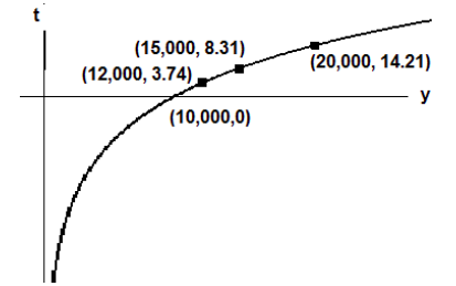
If we consider just the function \(\mathrm{t}=\mathrm{g}(\mathrm{y})=\frac{\ln \left(\frac{\mathrm{y}}{10000}\right)}{\ln (1.05)}\), then the domain of function would be \(y > 0\), all positive real numbers, and the range for \(t\) would be all real numbers.
In the context of this investment problem, the initial investment at time \(t\) = 0 is \(y\) =$10,000. Negative values for time do not make sense. Values of the investment that are lower than the initial amount of $10,000 also do not make sense for an investment that is increasing in value.
Therefore the function and graph as it pertains to this problem concerning investments has
domain \(y ≥ 10,000\) and range \(t ≥ 0\).
The graph below is restricted to the domain and range that make practical sense for the investment in this problem.