10.4: Absorbing Markov Chains

Learning Objectives

In this section, you will learn to:

1. Identify absorbing states and absorbing Markov chains
2. Solve and interpret absorbing Markov chains.

In this section, we will study a type of Markov chain in which when a certain state is reached, it is impossible to leave that state. Such states are called absorbing states, and a Markov Chain that has at least one such state is called an Absorbing Markov chain.

Suppose you have the following transition matrix.

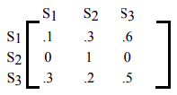
The state S₂ is an absorbing state, because the probability of moving from state S₂ to state S₂ is 1. Which is another way of saying that if you are in state S₂, you will remain in state S₂.

In fact, this is the way to identify an absorbing state. If the probability in row \(i\) and column \(i\), \(p_{ii}\), is 1, then state S_i is an absorbing state.

Example \(\PageIndex{1}\)

Consider transition matrices A, B, C for Markov chains shown below. Which of the following Markov chains have an absorbing state?

\[A=\left[\begin{array}{lll}
.3 & .7 & 0 \\
0 & 1 & 0 \\
.2 & .3 & .5
\end{array}\right] \quad B=\left[\begin{array}{lll}
0 & 1 & 0 \\
0 & 0 & 1 \\
1 & 0 & 0
\end{array}\right] \quad C=\left[\begin{array}{cccc}
.1 & .3 & .4 & .2 \\
0 & .2 & .1 & .7 \\
0 & 0 & 1 & 0 \\
0 & 0 & 0 & 1
\end{array}\right] \nonumber \]

Solution

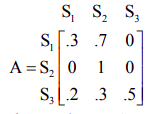has S₂ as an absorbing state.

If we are in state S₂, we can not leave it. From state S₂, we can not transition to state S₁ or S₃; the probabilities are 0.
The probability of transition from state S₂ to state S₂ is 1.

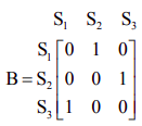does not have any absorbing states.

From state S₁, we always transition to state S₂. From state S₂ we always transition to state S₃. From state S₃ we always transition to state S₁. In this matrix, it is never possible to stay in the same state during a transition.

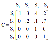has two absorbing states, S₃ and S₄.

From state S₃, you can only remain in state S₃, and never transition to any other states. Similarly from state S₄, you can only remain in state S₄, and never transition to any other states.

We summarize how to identify absorbing states.

Summary

A state S is an absorbing state in a Markov chain in the transition matrix if

• The row for state S has one 1 and all other entries are 0

AND

• The entry that is 1 is on the main diagonal (row = column for that entry), indicating that we can never leave that state once it is entered.

Next we define an absorbing Markov Chain

Absorbing Markov Chain

A Markov chain is an absorbing Markov Chain if

• It has at least one absorbing state

AND

• From any non-absorbing state in the Markov chain, it is possible to eventually move to some absorbing state (in one or more transitions).

Example \(\PageIndex{2}\)

Consider transition matrices C and D for Markov chains shown below. Which of the following Markov chains is an absorbing Markov Chain?

\[\mathrm{C}=\left[\begin{array}{llll}
.1 & .3 & .4 & .2 \\
0 & .2 & .1 & .7 \\
0 & 0 & 1 & 0 \\
0 & 0 & 0 & 1
\end{array}\right] \quad \mathrm{D}=\left[\begin{array}{lllll}
1 & 0 & 0 & 0 & 0 \\
0 & 1 & 0 & 0 & 0 \\
.2 & .2 & .2 & .2 & .2 \\
0 & 0 & 0 & .3 & .7 \\
0 & 0 & 0 & .6 & .4
\end{array}\right] \nonumber \]

Solution

C is an absorbing Markov Chain but D is not an absorbing Markov chain.

Matrix C has two absorbing states, S₃ and S₄, and it is possible to get to state S₃ and S₄ from S₁ and S₂.

Matrix D is not an absorbing Markov chain. It has two absorbing states, S₁ and S₂, but it is never possible to get to either of those absorbing states from either S₄ or S₅. If you are in state S₄ or S_5, you always remain transitioning between states S₄ or S_5m and can never get absorbed into either state S₁ or S₂

In the remainder of this section, we’ll examine absorbing Markov chains with two classic problems: the random drunkard’s walk problem and the gambler's ruin problem. And finally we’ll conclude with an absorbing Markov model applied to a real world situation.

Drunkard's Random Walk

In this example we briefly examine the basic ideas concerning absorbing Markov chains.

Example \(\PageIndex{3}\)

A man walks along a three block portion of Main St. His house is at one end of the three block section. A bar is at the other end of the three block section. Each time he reaches a corner he randomly either goes forward one block or turns around and goes back one block. If he reaches home or the bar, he stays there. The four states are Home (H), Corner 1(C₁), Corner 2 (C₂) and Bar (B).

Write the transition matrix and identify the absorbing states. Find the probabilities of ending up in each absorbing state depending on the initial state.

Solution

The transition matrix is written below.

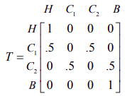
Home and the Bar are absorbing states. If the man arrives home, he does not leave. If the man arrives at the bar, he does not leave. Since it is possible to reach home or the bar from each of the other two corners on his walk, this is an absorbing Markov chain.

We can raise the transition matrix T to a high power, \(n\). One we find a power Tⁿ that remains stable, it will tell us the probability of ending up in each absorbing state depending on the initial state.

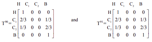
T⁹¹ = T⁹⁰; the matrix does not change as we continue to examine higher powers. We see that in the long-run, the Markov chain must end up in an absorbing state. In the long run, the man must eventually end up at either his home or the bar.

The second row tells us that if the man is at corner C₁, then there is a 2/3 chance he will end up at home and a 1/3 chance he will end up at the bar.

The third row tells us that if the man is at corner C₂, then there is a 1/3 chance he will end up at home and a 2/3 chance he will end up at the bar.

Once he reaches home or the bar, he never leaves that absorbing state.

Note that while the matrix Tⁿ for sufficiently large \(n\) has become stable and is not changing, it does not represent an equilibrium matrix. The rows are not all identical, as we found in the regular Markov chains that reached an equilibrium.

We can write a smaller “solution matrix” by retaining only rows that relate to the non-absorbing states and retaining only the columns that relate to the absorbing states.

Then the solution matrix will have rows C₁ and C₂, and columns H and B. The solution matrix is

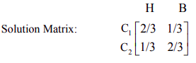
The first row of the solution matrix shows that if the man is at corner C₁, then there is a 2/3 chance he will end up at home and a 1/3 chance he will end up at the bar.

The second row of the solution matrix shows that if the man is at corner C₂, then there is a 1/3 chance he will end up at home and a 2/3 chance he will end up at the bar.

The solution matrix does not show that eventually there is 0 probability of ending up in C1 or C2, or that if you start in an absorbing state H or B, you stay there. The smaller solution matrix assumes that we understand these outcomes and does not include that information.

The next example is another classic example of an absorbing Markov chain. In the next example we examine more of the mathematical details behind the concept of the solution matrix.

Gamber's Ruin Problem

Example \(\PageIndex{4}\)

A gambler has $3,000, and she decides to gamble $1,000 at a time at a Black Jack table in a casino in Las Vegas. She has told herself that she will continue playing until she goes broke or has $5,000. Her probability of winning at Black Jack is .40. Write the transition matrix, identify the absorbing states, find the solution matrix, and determine the probability that the gambler will be financially ruined at a stage when she has $2,000.

Solution

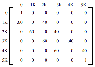
The transition matrix is written below. Clearly the state 0 and state 5K are the absorbing states. This makes sense because as soon as the gambler reaches 0, she is financially ruined and the game is over. Similarly, if the gambler reaches $5,000, she has promised herself to quit and, again, the game is over. The reader should note that p₀₀ = 1, and p₅₅ = 1.

Further observe that since the gambler bets only $1,000 at a time, she can raise or lower her money only by $1,000 at a time. In other words, if she has $2,000 now, after the next bet she can have $3,000 with a probability of .40 and $1,000 with a probability of .60.

To determine the long term trend, we raise the matrix to higher powers until all the non-absorbing states are absorbed. This is the called the solution matrix.

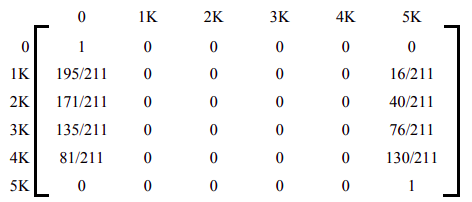
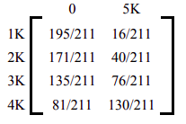
The solution matrix is often written in the following form, where the non-absorbing states are written as rows on the side, and the absorbing states as columns on the top.

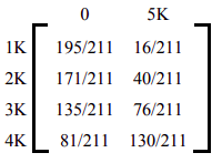
The table lists the probabilities of getting absorbed in state 0 or state 5K starting from any of the four non-absorbing states. For example, if at any instance the gambler has $3,000, then her probability of financial ruin is 135/211 and her probability reaching 5K is 76/211.

Example \(\PageIndex{5}\)

Solve the Gambler's Ruin Problem of Example \(\PageIndex{4}\) without raising the matrix to higher powers, and determine the number of bets the gambler makes before the game is over.

Solution

In solving absorbing states, it is often convenient to rearrange the matrix so that the rows and columns corresponding to the absorbing states are listed first. This is called the Canonical form. The transition matrix of Example 1 in the canonical form is listed below.

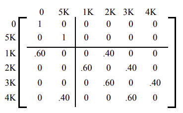
The canonical form divides the transition matrix into four sub-matrices as listed below.

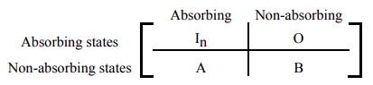
The matrix \(F = (I_n- B)^{-1}\) is called the fundamental matrix for the absorbing Markov chain, where In is an identity matrix of the same size as B. The \(i\), \(j\)-th entry of this matrix tells us the average number of times the process is in the non-absorbing state \(j\) before absorption if it started in the non-absorbing state \(i\).

The matrix \(F = (I_n- B)^{-1}\) for our problem is listed below.

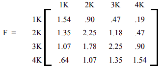
You can use your calculator, or a computer, to calculate matrix F.

The Fundamental matrix F helps us determine the average number of games played before absorption.

According to the matrix, the entry 1.78 in the row 3, column 2 position says that the gambler will play the game 1.78 times before she goes from $3K to $2K. The entry 2.25 in row 3, column 3 says that if the gambler now has $3K, she will have $3K on the average 2.25 times before the game is over.

We now address the question of how many bets will she have to make before she is absorbed, if the gambler begins with $3K?

If we add the number of games the gambler plays in each non-absorbing state, we get the average number of games before absorption from that state. Therefore, if the gambler starts with $3K, the average number of Black Jack games she will play before absorption is

\[1.07 + 1.78 + 2.25 + 0.90 = 6.0 \nonumber \]

That is, we expect the gambler will either have $5,000 or nothing on the 7th bet.

Lastly, we find the solution matrix without raising the transition matrix to higher powers. The matrix FA gives us the solution matrix.

\[\mathrm{FA}=\left[\begin{array}{cccc}
1.54 & .90 & .47 & .19 \\
1.35 & 2.25 & 1.18 & .47 \\
1.07 & 1.78 & 2.25 & .90 \\
.64 & 1.07 & 1.35 & 1.54
\end{array}\right]\left[\begin{array}{cc}
.6 & 0 \\
0 & 0 \\
0 & 0 \\
0 & .4
\end{array}\right]=\left[\begin{array}{cc}
.92 & .08 \\
.81 & .19 \\
.64 & .36 \\
.38 & .62
\end{array}\right] \nonumber \]

which is the same as the following matrix we obtained by raising the transition matrix to higher powers.

Example \(\PageIndex{6}\)

At a professional school, students need to take and pass an English writing/speech class in order to get their professional degree. Students must take the class during the first quarter that they enroll. If they do not pass the class they take it again in the second semester. If they fail twice, they are not permitted to retake it again, and so would be unable to earn their degree.

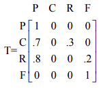
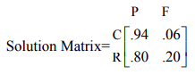
Students can be in one of 4 states: passed the class (P), enrolled in the class for the first time (C), retaking the class (R) or failed twice and can not retake (F). Experience shows 70% of students taking the class for the first time pass and 80% of students taking the class for the second time pass.

Write the transition matrix and identify the absorbing states. Find the probability of being absorbed eventually in each of the absorbing states.

Solution

The absorbing states are P (pass) and F (fail repeatedly and can not retake). The transition matrix T is shown below.

If we raise the transition matrix T to a high power, we find that it remains stable and gives us the long-term probabilities of ending up in each of the absorbing states.

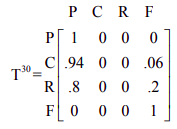
Of students currently taking the class for the first time, 94% will eventually pass. 6% will eventually fail twice and be unable to earn their degree.

Of students currently taking the class for the second time time, 80% will eventually pass. 20% will eventually fail twice and be unable to earn their degree.

The solution matrix contains the same information in abbreviated form

Note that in this particular problem, we don’t need to raise T to a “very high” power. If we find T², we see that it is actually equal to Tⁿ for higher powers \(n\). Tⁿ becomes stable after two transitions; this makes sense in this problem because after taking the class twice, the student must have passed or is not permitted to retake it any longer. Therefore the probabilities should not change any more after two transitions; by the end of two transitions, every student has reached an absorbing state.

Absorbing Markov Chains

1. A Markov chain is an absorbing Markov chain if it has at least one absorbing state. A state i is an absorbing state if once the system reaches state i, it stays in that state; that is, \(p_{ii} = 1\).
2. If a transition matrix T for an absorbing Markov chain is raised to higher powers, it reaches an absorbing state called the solution matrix and stays there. The \(i\), \(j\)-th entry of this matrix gives the probability of absorption in state \(j\) while starting in state \(i\).
3. Alternately, the solution matrix can be found in the following manner.
   1. Express the transition matrix in the canonical form as below. \[\mathrm{T}=\left[\begin{array}{ll}
      \mathbf{I}_{\mathbf{n}} & \mathbf{0} \\
      \mathbf{A} & \mathbf{B}
      \end{array}\right] \nonumber \] where \(I_n\) is an identity matrix, and 0 is a matrix of all zeros.
   2. The fundamental matrix \(F = (I - B)^{-1}\). The fundamental matrix helps us find the number of games played before absorption.
   3. FA is the solution matrix, whose \(i\), \(j\)-th entry gives the probability of absorption in state \(j\) while starting in state \(i\).
4. The sum of the entries of a row of the fundamental matrix gives us the expected number of steps before absorption for the non-absorbing state associated with that row.