6.3: Transforming Data Values

It is not at all unusual for the analyst to want to change the values that describe the relations between actors, or the values that describe the attributes of actors. Suppose the attribute "gender" had been entered into a data set using the values "1" and "2", and we wanted to change the attribute to be "Female" coded as "0" and "1". Or, suppose that we had recorded the strength of ties between companies by counting the number of members of boards of directors that they had in common. But we then decide that we are only interested in whether there are members in common or not. We need to change the coded values to be equal to "0" if there are no board members in common, and "1" if there are any (regardless of how many).

Just like statistical packages, UCINET has built-in tools that do some of the most common data transformations.

Transform>Recode is a very flexible and general purpose tool for recoding values in any UCINET data structure. Its dialog box has two tabs: "Files" and "Recode".

In the Files tab, you can browse for an input dataset, select which matrices in the set to recode (if there is more than one), which rows and columns to recode (this is good if you are working on a collection of attribute vectors, for example, and only want to recode selected ones), whether to recode the values on the diagonal, and the name of the output dataset.

In the Recode tab, you specify what you want done by creating rules. For example, if I wanted to recode all values 1, 2, and 3 to be zero; and any values of 4, 5, and 6 to be one, I would create two rules. "Values from 1 to 3 are recorded as 0." "Values from 4 to 6 are recoded as 1." The rules are created by using simple built-in tools.

Almost any transformation in a dataset of any complexity can be done with this tool. But, often there are simpler ways to do certain tasks.

Transform>Reverse recodes the values of selected rows, columns, and matrices so that the highest value is now the lowest, the lowest is now the highest, and all other values are linearly transformed. For example, the vector 1 3 3 5 6 would become the vector 6 4 4 2 1.

If we've coded a relationship as "strength of tie" but want our results to be about "weakness of tie" a "reverse" transform would be helpful.

Transform>Dichotomize is a tool that is useful for turning valued data into binary data. That is, if we have measured the strength of ties among actors (e.g. on a scale from 0 = no tie to 5 = strong tie), the "dichotomize" can be used to turn this into data that represent only the absence or presence of a tie (e.g. zero or one).

Why would one ever want to do this? To convert an ordinal or interval measure of relation strength into simple presence/absence may throw away considerable amounts of information. Many of the tools of social network analysis were developed for use with binary data only, and give misleading results (or none at all!) when applied to valued data. Many of the tools in UCINET that are designed for binary data will arbitrarily dichotomize interval or ordinal data in ways that might not be appropriate for your problem.

So, if your data are valued, but the tool you want to use requires binary data, you can turn your data into zero-one form by selecting a cut-off value (you will also have to select a "cut-off operator" and decide what to do with the diagonal).

Suppose, for example, I'd measured tie strength on a scale from 0 to 3. I'd like to have the values 0 and 1 treated as "0" and the values 2 and 3 treated as "1". I would select "greater than" as the cut-off operator, and select a cut-off value of "2". The result would be a binary matrix of zeros (when the original scores were 0 or 1) and ones (when the original scores were 2 or 3).

This tool can be particularly helpful when examining the values of many network measures. For example, the shortest distance between two actors ("geodesic distance") might be computed and saved in a file. We might then want to look at a map or image of the data at various levels of distance -- first, only display actors who are adjacent (distance = 1), then actors who are one or two steps apart, etc. The "dichotomize" tool could be used to create the necessary matrices.

Transform>Diagonal lets you modify the values of the ties of actors with themselves, or the "main diagonal" of square network data sets. The dialog box for this tool allows you to specify either a single value that is to be entered for all the cells on the diagonal; or, a list of (comma separated) values for each of the diagonal cells (from actor one through the last listed actor).

For many network analyses, the values on the main diagonal are not very meaningful, and you may wish to set them all to zero or to one -- which are pretty common approaches. Many of the tools for calculating network measures in UCINET will automatically ignore the main diagonal, or ask you whether to include it or not.

On some occasions, though, you may wish to be sure that ties of an actor with themselves are treated as present (e.g.set diagonal values to 1), or treated as absent (e.g. set diagonal values to zero).

Transform>Symmetrize is a tool that is used to turn "directed" or "asymmetric" network data into "un-directed" or "symmetric" data.

Many of the measures of network properties computed by UCINET are defined only for symmetric data (see the help screens for information about this). If you ask to calculate a measure that is defined for only symmetric data, but your data are not symmetric, UCINET either will refuse to calculate a measure, or will symmetrize the data for you.

But, there are a number of ways to symmetrize data, and you need to be sure that you choose an approach that makes sense for your particular problem. The choices that are available in the Transform>Symmetrize tool are:

>Maximum looks at each cell in the upper part of the matrix and the corresponding cell in the lower part of the matrix (e.g. cell 2,5 is compared to cell 5,2), and enters the larger of the values found into both cells (e.g. 2,5 and 5,2 will now have the same output value). For example, suppose that we felt that the strength of the tie between actor A and actor B was best represented as being the strongest of the ties between them (either A's tie to B, or B's tie to A, whichever was strongest).

>Minimum characterizes the strength of the symmetric tie between A and B as being the weaker of the ties AB or BA. This corresponds to the "weakest link", and is a pretty common choice.

>Average characterizes the strength of the symmetric tie between A and B as the simple average of the ties AB and BA. Honestly, I have trouble thinking of a case where this approach makes a lot of sense for social relations.

>Sum characterizes the strength of the symmetric tie between A and B as the sum of AB and BA. This does make some sense -- that all the tie strength be included, regardless of direction.

>Difference characterizes the strength of the symmetric tie between A and B as |AB - BA|. So, relationships that are completely reciprocal end up with a value of zero; those that are completely asymmetric end up with a value equal to the stronger relation.

>Product characterizes the strength of the symmetric relation between A and B as the product of AB and BA. If reciprocity is necessary for us to regard a relationship as being "strong" then either "sum" or "product" might be a logical approach to symmetrizing.

>Division characterizes the strength of the symmetric relation between A and B as AB/BA. This approach "penalizes" relations that are equally reciprocated, and "rewards" relations that are strong in one direction, but not the other.

>Lower Half or >Upper Half uses the values in one half of the matrix for the other half. For example, the value of BA is set equal to whatever AB is. This transformation, though it may seem odd at first, is quite helpful. If we are interested in focusing on the network properties of "senders" we would choose to set the lower half equal to the upper half (i.e. select Upper Half). If we were interested in the structure of tie receiving, we would set the upper half equal to the lower.

>Upper > Lower or >Upper < Lower (and similar functions available in the dialog box) compare the values in cell AB and BA, and return one or the other based on the test function. If, for example, we had selected Upper > Lower and AB = 3 and BA = 5, the function would select the value "5", because the upper value (AB) was not greater than the lower value (BA).

Transform>Normalize provides a number of tools for rescaling the scores in rows, in columns, or in both dimensions of a matrix of valued relations. A simple example might be helpful.

Figure 6.4 shows some data (from the United Nations Commodity Trade database) on trade flows, valued in dollars, of softwood lumber among 5 major Pacific Rim nations at c. 2000.

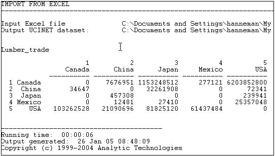
Figure 6.4: Value of softwood lumber exports among five nations.

Suppose we were interested in exploring the structure of export partner dependence -- the disadvantage that a nation might face in establishing high prices when it has few alternative places to sell its products. For this purpose, we might choose to "normalize" the data by expressing it as row percentages.That is, what proportion of Canada's exports went to China, Japan, etc. Using the row normalization routine, we produce Figure 6.5.

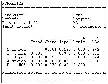
Figure 6.5: Row (sending or export) normalized lumber trade data.

Graphing the original trade-flow data would answer our question, but graphing the row normalized data gives us a much clearer picture of export dependency. If we were interested in import partner trading concentration, we might normalize the data by columns, producing Figure 6.6.

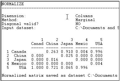
Figure 6.6: Column (receiving or import) normalized lumber trade data.

We see, for example, that all of Canada's imports are from the USA, and that virtually all of the USA's imports are from Canada.

The >Transform>Normalize tool provides a number of ways of re-scaling the data that are frequently used.

Normalization may be applied to either rows or columns (as in our examples, above), or it may be applied to the entire matrix (for example, rescaling all trade flows as percentages of the total amount of trade flow in the whole matrix). Normalization may also be applied to both rows and columns, iteratively. For example, if we wanted an "average" number to put in each cell of the trade flow matrix, so that both the rows and the columns summed to \(100\%\), we could apply the iterative row and column approach. This is sometimes used when we want to give "equal weight" to each node, and to take into account both outflow (row) and inflow (column) structure.

There are a number of alternative, commonly used, approaches to how to rescale the data. Our examples use the "marginal" total (row or column) and set the sum of the entries in each row (or column) to equal 1.0. Alternatively, we might want to express each entry relative to the mean score (e.g.divide each element of the row by the average of the elements in a row). Alternatively, one might rescale by dividing by the standard deviation, or both mean and standard deviation (i.e. express the elements as Z scores). UCINET supports all of these as built-in functions. In addition, scores can be normalized by Euclidean norm, or by expressing each element as a percentage of the maximum element in a row.

Rescaling transforms like these can be very, very helpful in highlighting structural features of the data. But, obviously different normalizing approaches highlight very different features. Try thinking through how what applying each of the available transformations would tell you for some data that describe a relation that you are interested in. Some of the transformations will be completely useless; some may give you some new ideas.