5.2: 5.2 Phase Space Visualization of Continuous-State Discrete-Time Models

Last updated
Save as PDF

Page ID: 7790

$ \newcommand{\vecs}[1]{\overset { \scriptstyle \rightharpoonup} {\mathbf{#1}} } $ $ \newcommand{\vecd}[1]{\overset{-\!-\!\rightharpoonup}{\vphantom{a}\smash {#1}}} $$\newcommand{\id}{\mathrm{id}}$ $ \newcommand{\Span}{\mathrm{span}}$ $ \newcommand{\kernel}{\mathrm{null}\,}$ $ \newcommand{\range}{\mathrm{range}\,}$ $ \newcommand{\RealPart}{\mathrm{Re}}$ $ \newcommand{\ImaginaryPart}{\mathrm{Im}}$ $ \newcommand{\Argument}{\mathrm{Arg}}$ $ \newcommand{\norm}[1]{\| #1 \|}$ $ \newcommand{\inner}[2]{\langle #1, #2 \rangle}$ $ \newcommand{\Span}{\mathrm{span}}$ $\newcommand{\id}{\mathrm{id}}$ $ \newcommand{\Span}{\mathrm{span}}$ $ \newcommand{\kernel}{\mathrm{null}\,}$ $ \newcommand{\range}{\mathrm{range}\,}$ $ \newcommand{\RealPart}{\mathrm{Re}}$ $ \newcommand{\ImaginaryPart}{\mathrm{Im}}$ $ \newcommand{\Argument}{\mathrm{Arg}}$ $ \newcommand{\norm}[1]{\| #1 \|}$ $ \newcommand{\inner}[2]{\langle #1, #2 \rangle}$ $ \newcommand{\Span}{\mathrm{span}}$$\newcommand{\AA}{\unicode[.8,0]{x212B}}$

Once you find where the equilibrium points of the system are, the next natural step of analysis would be to draw the entire picture of its phase space (if the system is two or three dimensional).

For discrete-time systems with continuous-state variables (i.e., state variables that take real values), drawing a phase space can be done very easily using straightforward computer simulations, just like we did in Fig. 4.4.2. To reveal a large-scale structure of the phase space, however, you will probably need to draw many simulation results starting from different initial states. This can be achieved by modifying the initialization function so that it can receive specific initial values for state variables, and then you can put the simulation code into for loops that sweep the parameter values for a given range. For example:

$Code 5.1.png$

$Code 5.1 pt2.png$

$Code 5.1 pt3.png$
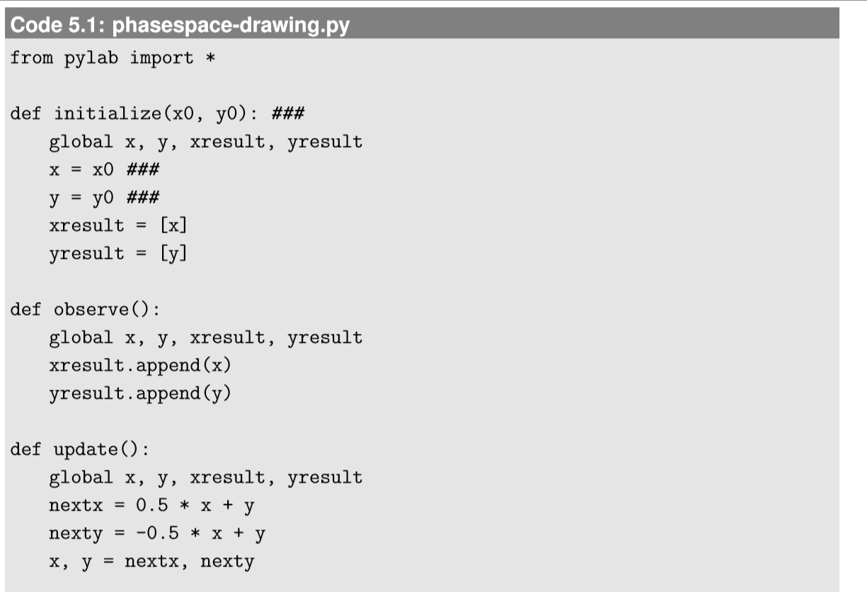
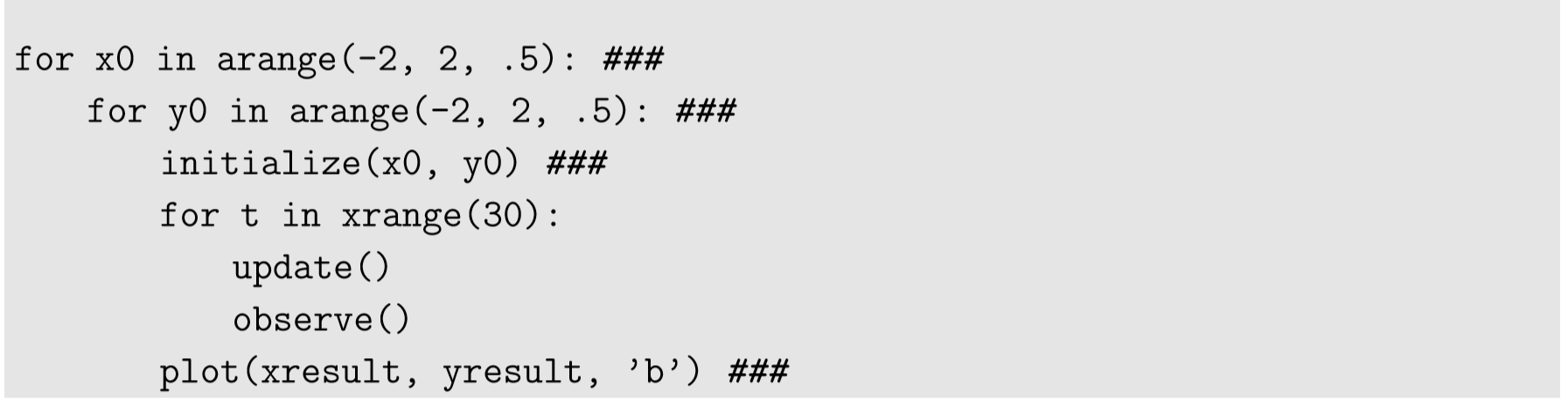
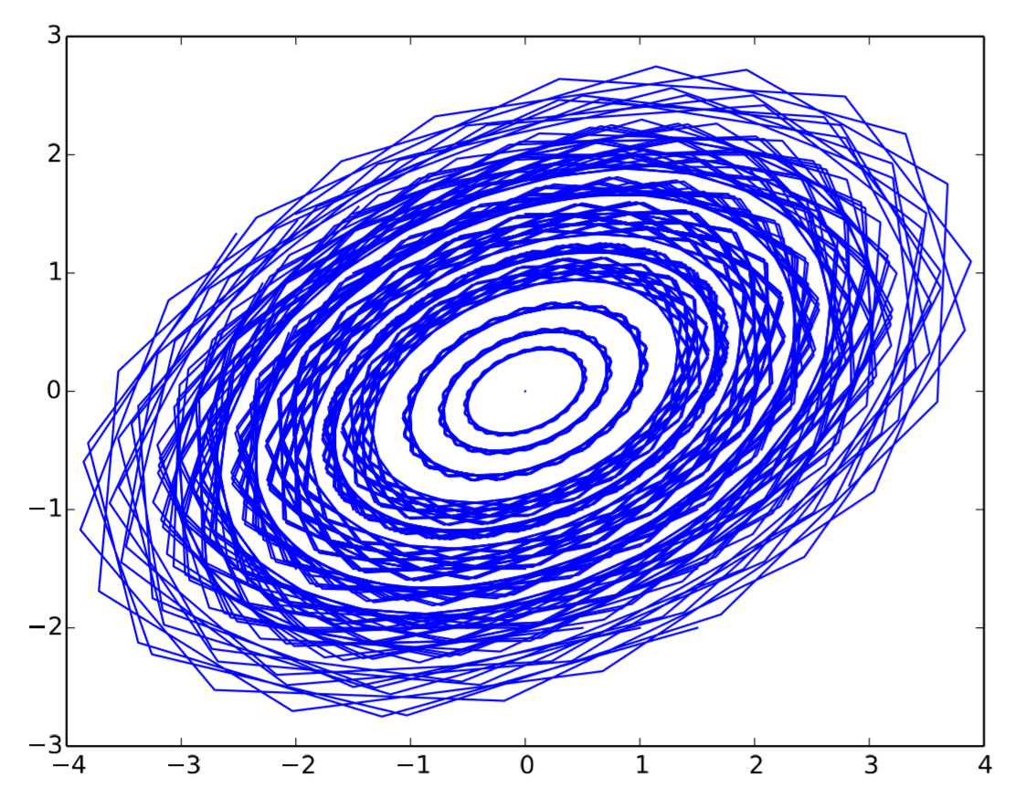
Revised parts from the previous example are marked with ###. Here, the arange function was used to vary initial x and y values over $[−2,2]$ at interval 0.5. For each initial state, a simulation is conducted for 30 steps, and then the result is plotted in blue (the ’b’ option of plot). The output of this code is Fig. 5.2.1, which clearly shows that the phase space of this system is made of many concentric trajectories around the origin.

Fig. 5.1.PNG — Figure $\PageIndex{1}$: Phase space drawn using Code 5.1.

Exercise $\PageIndex{1}$

Draw a phase space of the following two-dimensional difference equation model in Python:

\[x_{t} = x_{t-1} +0.1(x_{t-1} -x_{t-1}y_{t-1})\label{(5.11)} \]

\[y_{t} =y_{t-1} +0.1(y_{t-1} -x_{t-1}y_{t-1})\label{(5.12)} \]

\[(x>0, x>0)\label{(5.13)} \]

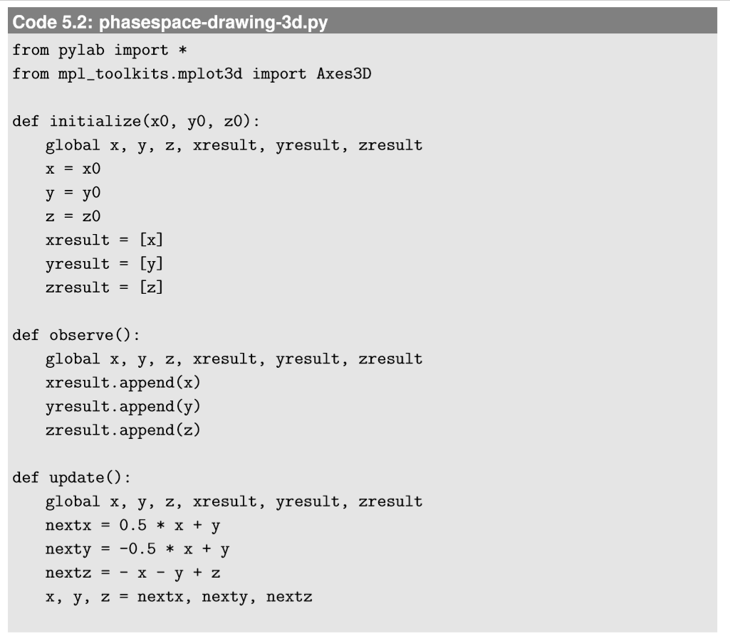
Three-dimensional systems can also be visualized in a similar manner. For example, let’s try visualizing the following three-dimensional difference equation model:

\[x_{t} =0.5x+y\label{(5.14)} \]

\[y_{t} =-0.5x +y\label{(5.15)} \]

\[z_{t} = -x-y+z\label{(5.16)} \]

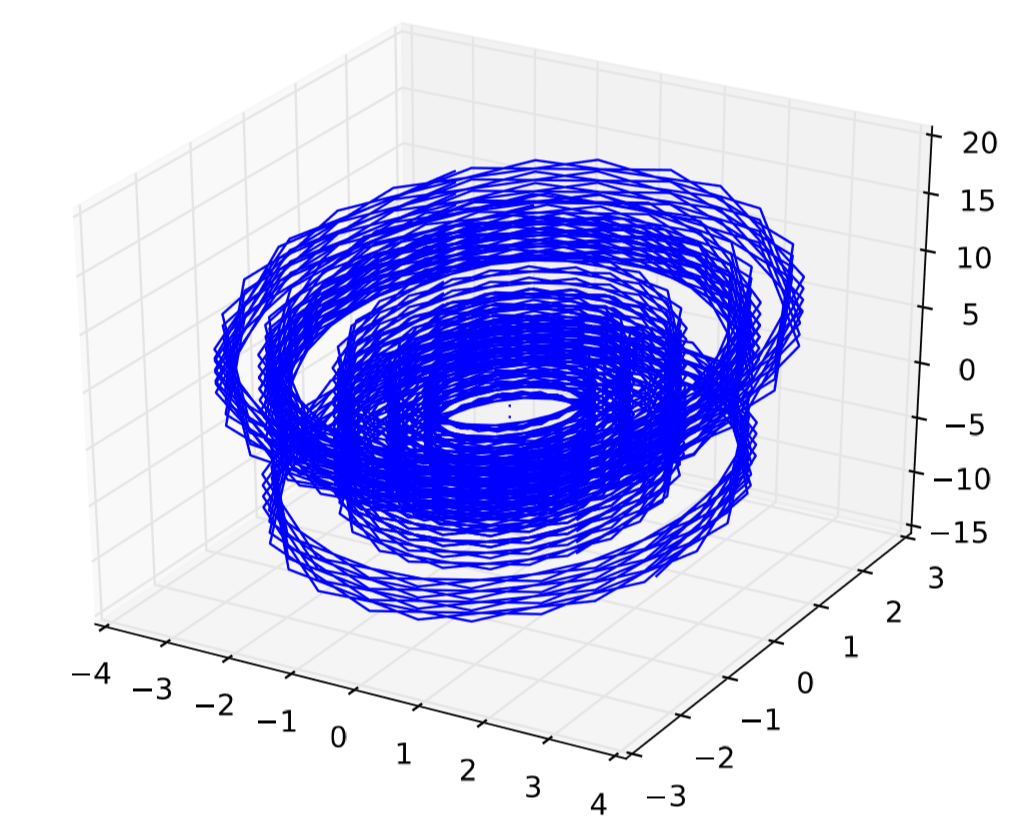
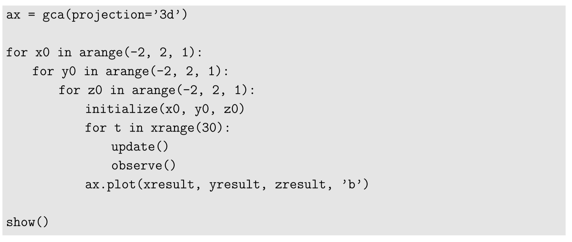
Plotting in 3-D requires an additional matplotlib component called Axes3D. A sample code is given in Code 5.2. Note the new import Axes3D line at the beginning, as well as the two additional lines before the for loops. This code produces the result shown in Fig. 5.2.2.

$Code 5.2.png$

$Code 5.2 pt.png$

Note that it is generally not a good idea to draw many trajectories in a 3-D phase space, because the visualization would become very crowded and difficult to see. Drawing a small number of characteristic trajectories is more useful.

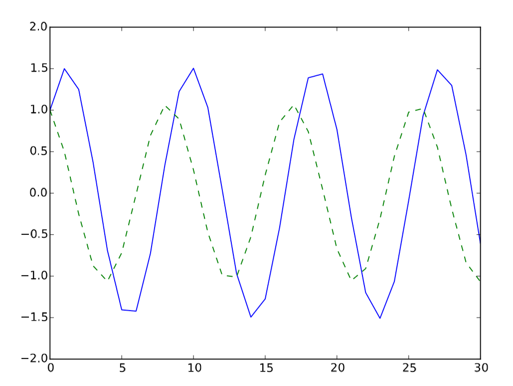
In general, you should keep in mind that phase space visualization of discrete-time models may not always give images that are easily visible to human eye. This is because the state of a discrete-time system can jump around in the phase space, and thus the trajectories can cross over each other (this will not happen for continuous-time models). Here is an example. Replace the content of the update function in Code 5.1 with the following:

$code 5.3.png$
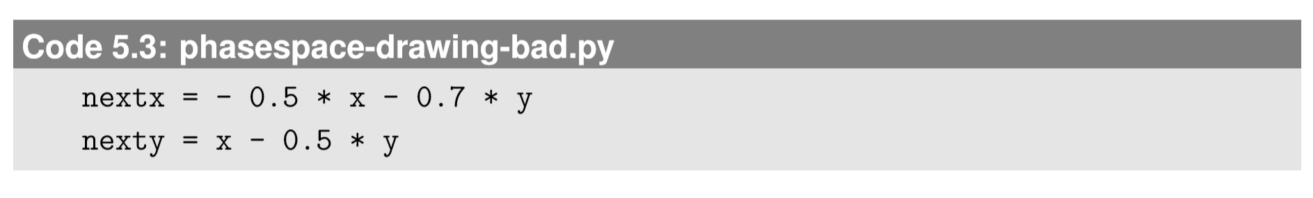
As a result, you get Fig. 5.2.3. While this may be aesthetically pleasing, it doesn’t help our understanding of the system very much because there are just too many trajectories overlaid in the diagram. In this sense, the straightforward phase space visualization may not always be helpful for analyzing discrete-time dynamical systems. In the following sections, we will discuss a few possible workarounds for this problem.

Fig. 5.2.PNG — Figure $\PageIndex{2}$: Three-dimensional phase space drawn with Code 5.2. If you are drawing this from an interactive environment, such as Anaconda Spyder or Enthought Canopy, you can rotate the 3-D plot interactively by clicking and dragging.

Figure $\PageIndex{3}$: Phase space drawn with Code 5.3.