15.2: Terminologies of Graph Theory

Last updated
Save as PDF

Page ID: 7858

$ \newcommand{\vecs}[1]{\overset { \scriptstyle \rightharpoonup} {\mathbf{#1}} } $ $ \newcommand{\vecd}[1]{\overset{-\!-\!\rightharpoonup}{\vphantom{a}\smash {#1}}} $$\newcommand{\id}{\mathrm{id}}$ $ \newcommand{\Span}{\mathrm{span}}$ $ \newcommand{\kernel}{\mathrm{null}\,}$ $ \newcommand{\range}{\mathrm{range}\,}$ $ \newcommand{\RealPart}{\mathrm{Re}}$ $ \newcommand{\ImaginaryPart}{\mathrm{Im}}$ $ \newcommand{\Argument}{\mathrm{Arg}}$ $ \newcommand{\norm}[1]{\| #1 \|}$ $ \newcommand{\inner}[2]{\langle #1, #2 \rangle}$ $ \newcommand{\Span}{\mathrm{span}}$ $\newcommand{\id}{\mathrm{id}}$ $ \newcommand{\Span}{\mathrm{span}}$ $ \newcommand{\kernel}{\mathrm{null}\,}$ $ \newcommand{\range}{\mathrm{range}\,}$ $ \newcommand{\RealPart}{\mathrm{Re}}$ $ \newcommand{\ImaginaryPart}{\mathrm{Im}}$ $ \newcommand{\Argument}{\mathrm{Arg}}$ $ \newcommand{\norm}[1]{\| #1 \|}$ $ \newcommand{\inner}[2]{\langle #1, #2 \rangle}$ $ \newcommand{\Span}{\mathrm{span}}$$\newcommand{\AA}{\unicode[.8,0]{x212B}}$

Before moving on to actual dynamical network modeling, we need to cover some basics of graph theory, especially the definitions of technical terms used in this field. Let’s begin with something we have already discussed above:

A network (or graph) consists of a set of nodes (or vertices, actors) and a set of edges (or links, ties) that connect those nodes.

As indicated above, different disciplines use different terminologies to talk about networks; mathematicians use “graph/vertex/edge,” physicists use “network/node/edge,” computer scientists use “network/node/link,” social scientists use “network/actor/tie,” etc. This is a typical problem when you work in an interdisciplinary research area like network science. We just need to get used to it. In this textbook, I mostly use “network/node/edge” or “network/node/link,” but I may sometimes use other terms interchangeably as well.

By the way, some people ask what are the differences between a “network” and a “graph.” I would say that a “network” implies it is a model of something real, while a “graph” emphasizes more on the aspects as an abstract mathematical object (which can also be used as a model of something real, of course). But this distinction isn’t so essential either.

To represent a network, we need to specify its nodes and edges. One useful term is neighbor, defined as follows:

Node $j$ is called a neighbor of node $i$ if (and only if) node $i$ is connected to node $j$.

The idea of neighbors is particularly helpful when we attempt to relate network models with more classical models such as CA (where neighborhood structures were assumed regular and homogeneous). Using this term, we can say that the goal of network representation is to represent neighborhood relationships among nodes. There are many different ways of representing networks, but the following two are the most common:

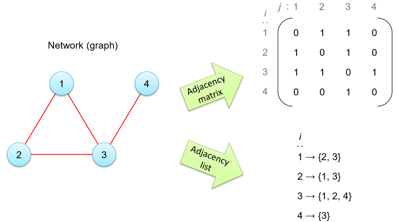
Adjacency matrix A matrix with rows and columns labeled by nodes, whose $i$-th row, $j$-th column component $a_{ij}$ is 1 if node $i $ is a neighbor of node $j$, or 0 otherwise.

Adjacency list A list of lists of nodes whose $i$-th component is the list of node $i$’s neighbors.

Figure15.1 shows an example of the adjacency matrix/list. As you can see, the adjacency list offers a more compact, memory-efficient representation, especially if the network is sparse (i.e., if the network density is low—which is often the case for most real-world networks). In the meantime, the adjacency matrix also has some benefits, such as its feasibility for mathematical analysis and easiness of having access to its specific components.

Here are some more basic terminologies:

Degree The number of edges connected to a node. Node $i$’s degree is often written as $deg(i)$.

Fig 15.1.png — Figure $\PageIndex{1}$: Examples of an adjacent matrix and an adjacent list.

Walk A list of edges that are sequentially connected to form a continuous route on a network. In particular:
Trail A walk that doesn’t go through any edge more than once.
Path A walk that doesn’t go through any node (and therefore any edge, too) more than once.
Cycle A walk that starts and ends at the same node without going through any node more than once on its way.
Subgraph Part of the graph.
Connected graph A graph in which a path exists between any pair of nodes.
Connected component A subgraph of a graph that is connected within itself but not connected to the rest of the graph.

Exercise $\PageIndex{1}$

See the following network and answer the following questions:

$Ex 15.1.png$

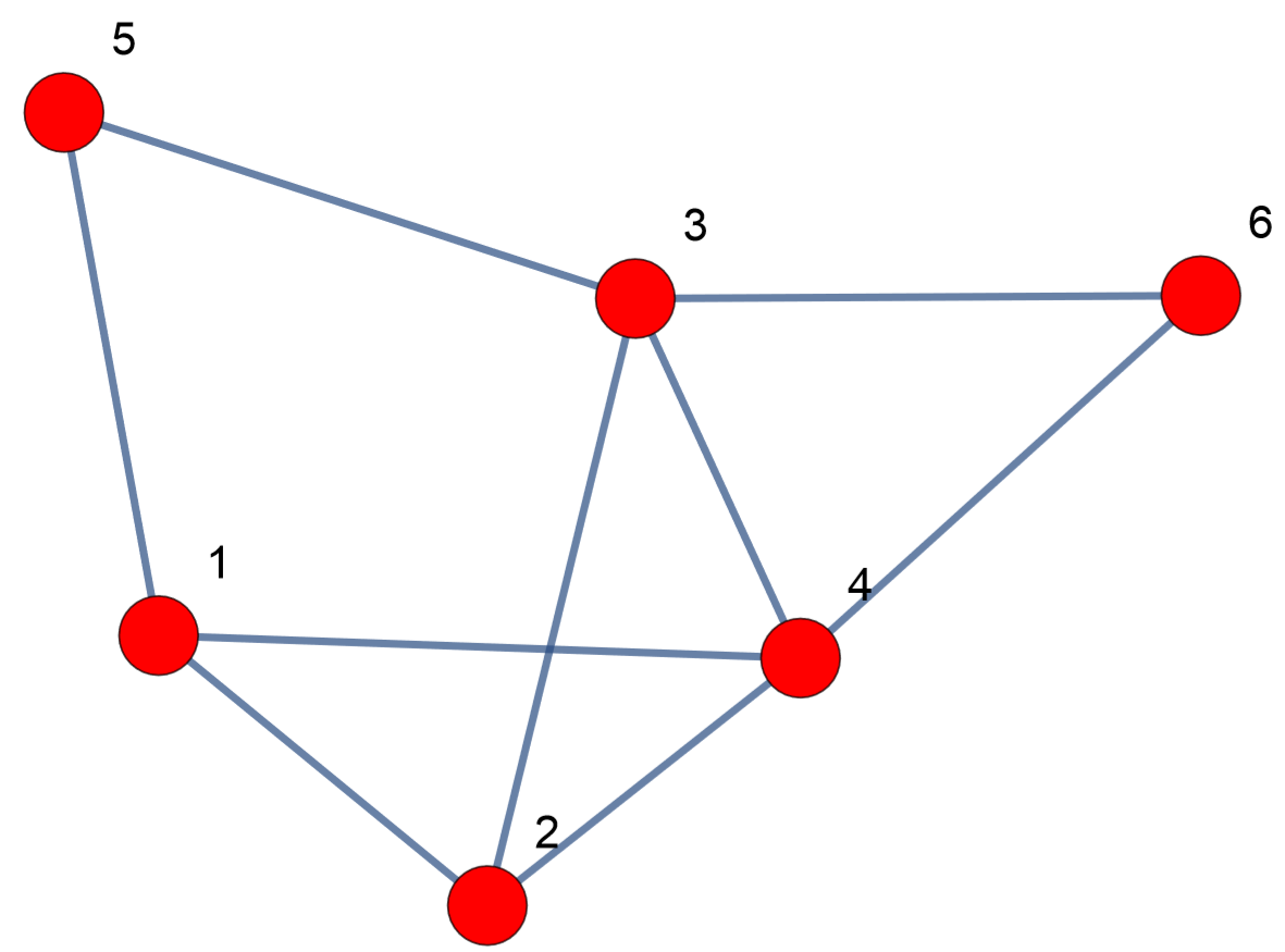
1. Represent the network in (a) an adjacency matrix, and (b) an adjacency list.

2. Determine the degree for each node.

3. Classify the following walks as trail, path, cycle, or other.

6 → 3 → 2 → 4 → 2 → 1
1 → 4 → 6 → 3 → 2
5 → 1 → 2 → 3 → 5

4. Identify all fully connected three-node subgraphs (i.e., triangles).

5. Remove nodes 3 and 4 (and all edges connected to them). Then identify the connected components in the resulting graph.

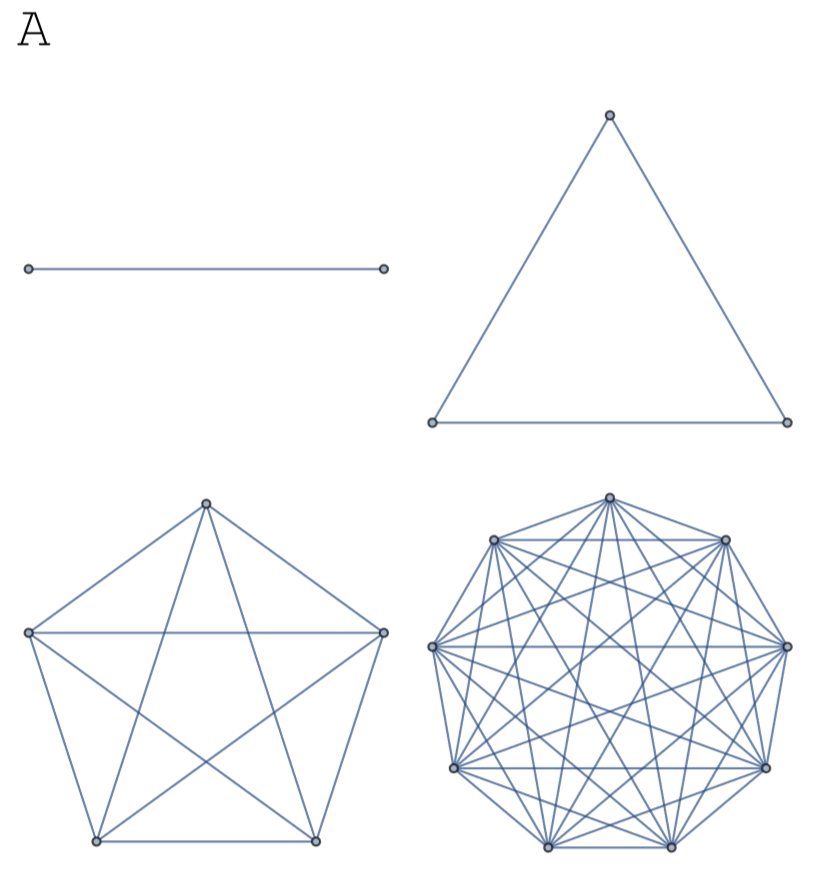
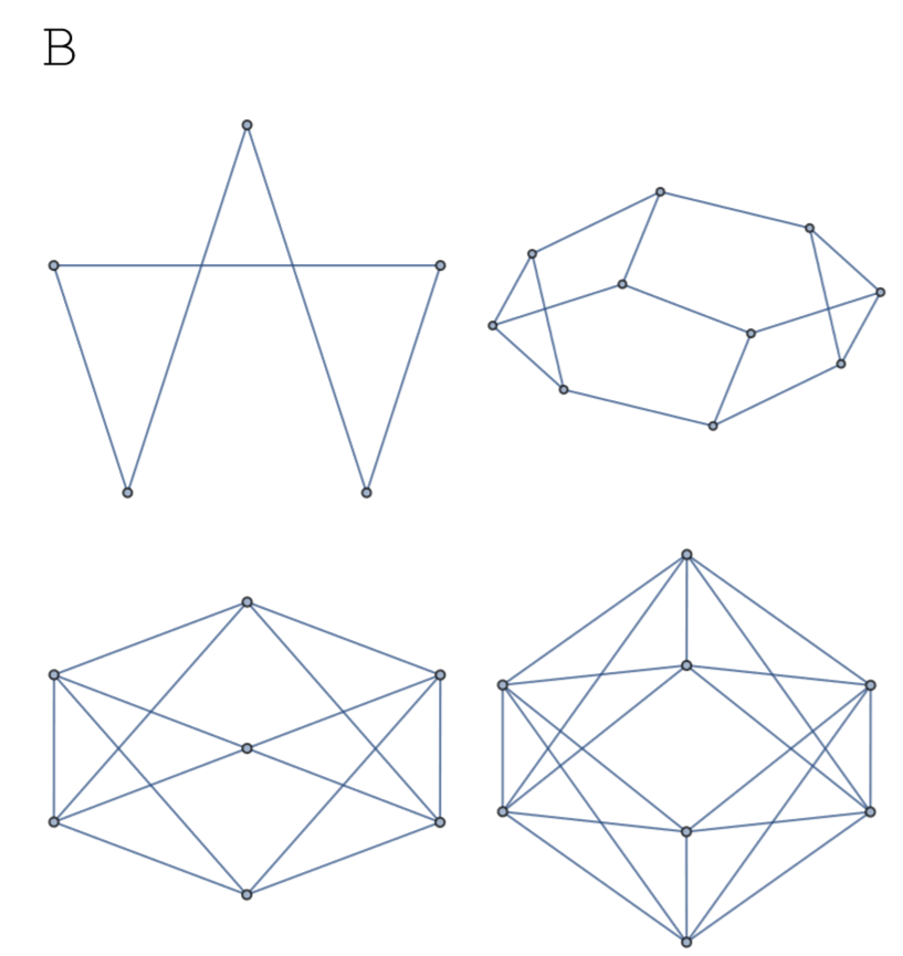
Some graphs with characteristic topological properties are given their own unique names, as follows

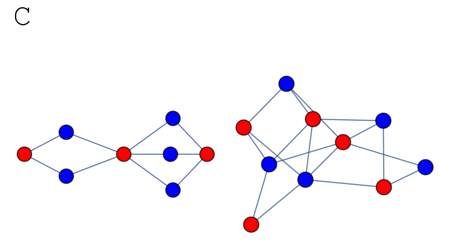
Complete graph A graph in which any pair of nodes are connected (Fig. 15.2.2A).
Regular graph A graph in which all nodes have the same degree(Fig.15.2.2B).Every complete graph is regular.
Bipartite ($n$ -partite) graph A graph whose nodes can be divided into two (or $n$) groups so that no edge connects nodes within each group (Fig. 15.2.2C).
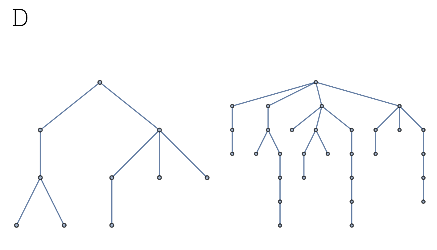
Tree graph A graph in which there is no cycle (Fig. 15.2.2D). A graph made of multiple trees is called a forest graph. Every tree or forest graph is bipartite.
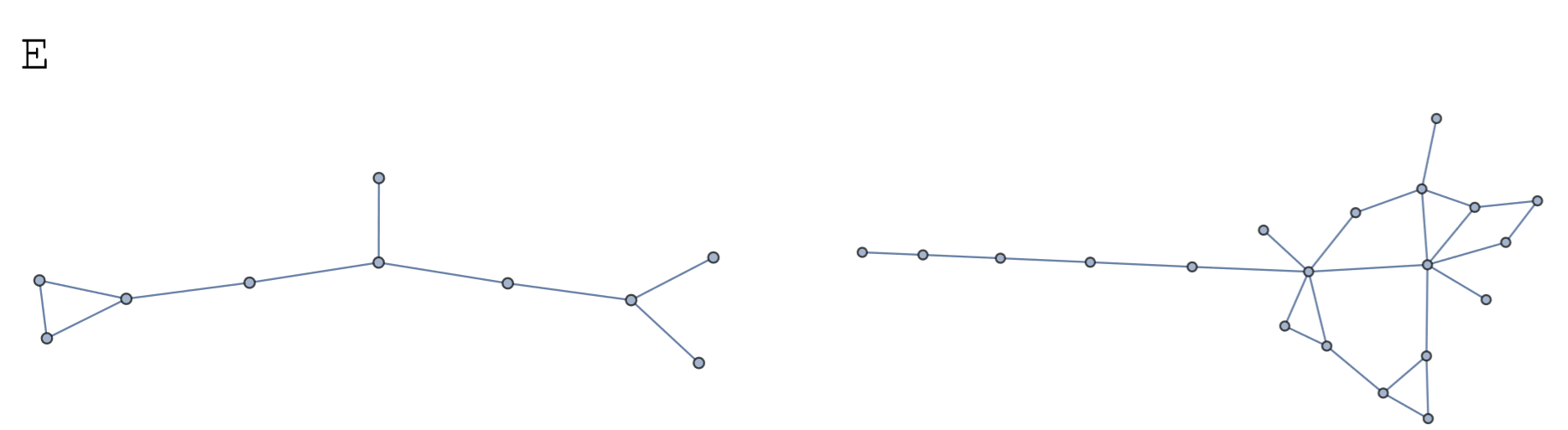
Planar graph A graph that can be graphically drawn in a two-dimensional plane with no edge crossings (Fig. 15.2.2E). Every tree or forest graph is planar.

$Fig. 15.2 A.PNG$ $Fig. 15.2B.PNG$

$Fig. 15.2C.PNG$ $Fig. 15.2D.PNG$

Fig. 15.2E.PNG — Figure $\PageIndex{2}$: Examples of graphs with specific names. A: Complete graphs. B:Regular graphs. C: Bipartite graphs (colors show groups). D: Tree graphs. E: Planar graphs.

Exercise $\PageIndex{2}$

Calculate the following:

The number of edges in a complete graph made of $n$ nodes
The number of edges in a regular graph made of $n$ nodes each of which has degree $k$

Exercise $\PageIndex{3}$

Determine whether the following graphs are planar or not:

A complete graph made of four nodes
A complete graph made of five nodes
A bipartite graph made of a two-node group and a three-node group in which all possible inter-group edges are present
A bipartite graph made of two three-node groups in which all possible intergroup edges are present

Exercise $\PageIndex{4}$

Every connected tree graph made of $n$ nodes has exactly $n − 1$edges. Explain why.

There are also classifications of graphs according to the types of their edges:

Undirected edge A symmetric connection between nodes. If node $i$ is connected to node $j$ by an undirected edge, then node $j$ also recognizes node $i$ as its neighbor. A graph made of undirected edges is called an undirected graph. The adjacency matrix of an undirected graph is always symmetric.
Directed edge An asymmetric connection from one node to another. Even if node $i$ is connected to node $j$ by a directed edge, the connection isn’t necessarily reciprocated from node $j$ to node $i$. A graph made of directed edges is called a directed graph. The adjacency matrix of a directed graph is generally asymmetric.
Unweighted edge An edge without any weight value associated to it. There are only two possibilities between a pair of nodes in a network with unweighted edges; whether there is an edge between them or not. The adjacency matrix of such a network is made of only 0’s and 1’s.
Weighted edge An edge with a weight value associated to it. A weight is usually given by a non-negative real number, which may represent a connection strength or distance between nodes, depending on the nature of the system being modeled. The definition of the adjacency matrix can be extended to contain those edge weight values for networks with weighted edges. The sum of the weights of edges connected to a node is often called the node strength, which corresponds to a node degree for unweighted graphs.
Multiple edges Edges that share the same origin and destination. Such multiple edges connect two nodes more than once.
Self-loop An edge that originates and ends at the same node.
Simple graph A graph that doesn’t contain directed, weighted, or multiple edges, or self-loops. Traditional graph theory mostly focuses on simple graphs.
Multigraph A graph that may contain multiple edges. Many mathematicians also allow multigraphs to contain self-loops. Multigraphs can be undirected or directed.
Hyperedge A generalized concept of an edge that can connect any number of nodes at once, not just two. A graph made of hyperedges is called a hypergraph (not covered in this textbook).

According to these taxonomies, all the examples shown in Fig. 15.2.2 are simple graphs. But many real-world networks can and should be modeled using directed, weighted, and/or multiple edges

Exercise $\PageIndex{5}$

Discuss which type of graph should be used to model each of the following networks. Make sure to consider (a) edge directedness, (b) presence of edge weights, (c) possibility of multiple edges/self-loops, (d) possibility of connections among three or more nodes, and so on.

Family trees/genealogies
Food webs among species
Roads and intersections
Web pages and links among them
Friendships among people
Marriages/sexual relationships
College applications submitted by high school students
Email exchanges among coworkers
Social media (Facebook, Twitter, Instagram, etc.)

Exercise \(\PageIndex{1}\)

Exercise \(\PageIndex{2}\)

Exercise \(\PageIndex{3}\)

Exercise \(\PageIndex{4}\)

Exercise \(\PageIndex{5}\)