17.1: Network Size, Density, and Percolation

Last updated
Save as PDF

Page ID: 7871

$ \newcommand{\vecs}[1]{\overset { \scriptstyle \rightharpoonup} {\mathbf{#1}} } $ $ \newcommand{\vecd}[1]{\overset{-\!-\!\rightharpoonup}{\vphantom{a}\smash {#1}}} $$\newcommand{\id}{\mathrm{id}}$ $ \newcommand{\Span}{\mathrm{span}}$ $ \newcommand{\kernel}{\mathrm{null}\,}$ $ \newcommand{\range}{\mathrm{range}\,}$ $ \newcommand{\RealPart}{\mathrm{Re}}$ $ \newcommand{\ImaginaryPart}{\mathrm{Im}}$ $ \newcommand{\Argument}{\mathrm{Arg}}$ $ \newcommand{\norm}[1]{\| #1 \|}$ $ \newcommand{\inner}[2]{\langle #1, #2 \rangle}$ $ \newcommand{\Span}{\mathrm{span}}$ $\newcommand{\id}{\mathrm{id}}$ $ \newcommand{\Span}{\mathrm{span}}$ $ \newcommand{\kernel}{\mathrm{null}\,}$ $ \newcommand{\range}{\mathrm{range}\,}$ $ \newcommand{\RealPart}{\mathrm{Re}}$ $ \newcommand{\ImaginaryPart}{\mathrm{Im}}$ $ \newcommand{\Argument}{\mathrm{Arg}}$ $ \newcommand{\norm}[1]{\| #1 \|}$ $ \newcommand{\inner}[2]{\langle #1, #2 \rangle}$ $ \newcommand{\Span}{\mathrm{span}}$$\newcommand{\AA}{\unicode[.8,0]{x212B}}$

Networks can be analyzed in several different ways. One way is to analyze their structural features, such as size, density, topology, and statistical properties.

Let me first begin with the most basic structural properties, i.e., the size and density of a network. These properties are conceptually similar to the mass and composition of matter—they just tell us how much stuff is in it, but they don’t tell us anything about how the matter is organized internally. Nonetheless, they are still the most fundamental characteristics, which are particularly important when you want to compare multiple networks. You should compare properties of two networks of the same size and density, just like chemists who compare properties of gold and copper of the same mass.

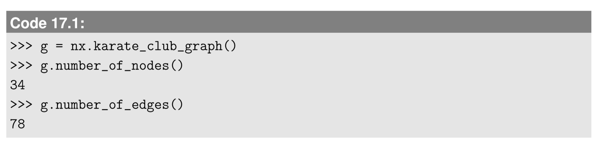
The size of a network is characterized by the numbers of nodes and edges in it.

NetworkX’s Graph objects have functions dedicated for measuring those properties:
$Code 17.1.PNG$

The density of a network is the fraction between 0 and 1 that tells us what portion of all possible edges are actually realized in the network. For a network $G$ made of $n$ nodes and $m$ edges, the density $ρ(G)$ is given by

\[p(G) =\frac{m}{\frac{n(n-1)}{2}} =\frac{2m}{n(n-1)} \label{(17.1)} \]

for an undirected network, or
\[p(G)= \frac{m}{n-1}\label{(17/2)} \]

for a directed network.

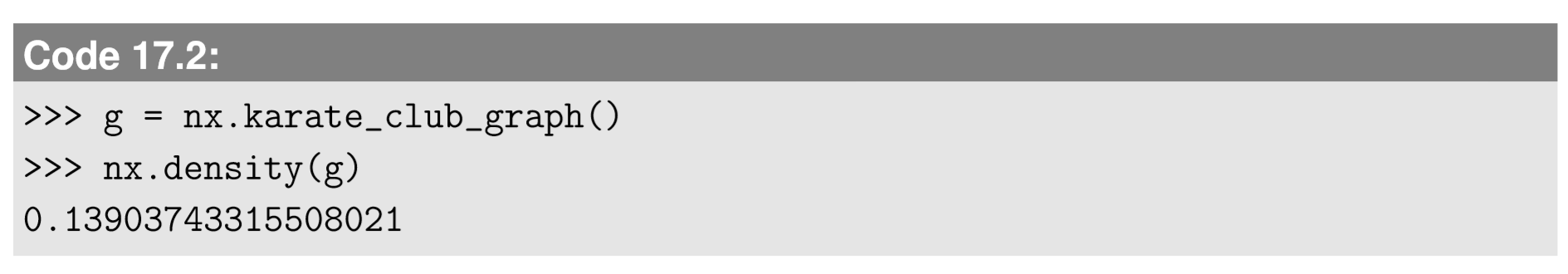
NetworkX has a built-in function to calculate network density:

$Code 17.2.PNG$

Note that the size and density of a network don’t specify much about the network’s actual topology(i.e.,shape). There are many networks with different topologies that have exactly the same size and density.

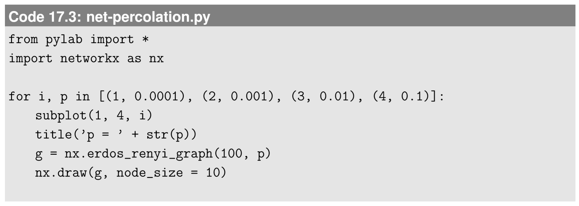
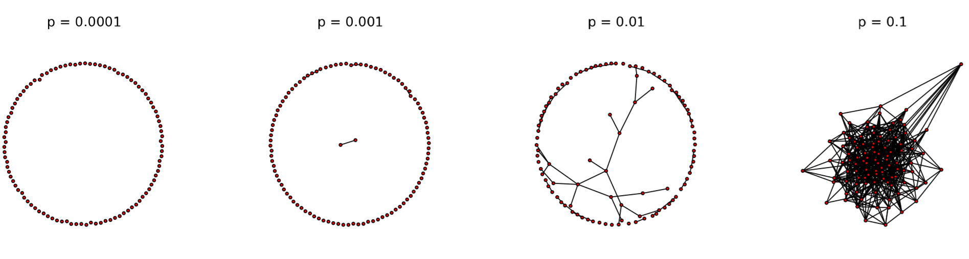
But there are some things the size and density can still predict about networks. One such example is network percolation, i.e., whether or not the nodes are sufficiently connected to each other so that they form a giant component that is visible at macroscopic scales. I can show you an example. In the code below, we generate Erd˝os-R´enyi random graphs made of 100 nodes with different connection probabilities:

$Code 17.3.PNG$

$Code 17.3 pt2.PNG$

The result is shown in Fig. 17.1.1, where we can clearly see a transition from a completely disconnected set of nodes to a single giant network that includes all nodes.

Fig 17.1.PNG — Figure $\PageIndex{1}$: Visual output of Code 17.3.

The following code conducts a more systematic parameter sweep of the connection probability:

$Code 17.4 pt1.PNG$

$Code 17.4 pt2.PNG$

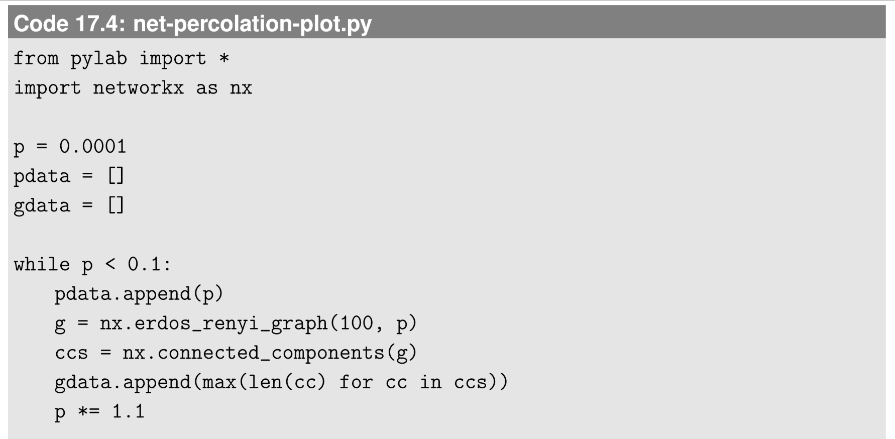
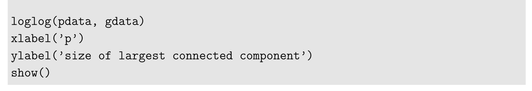
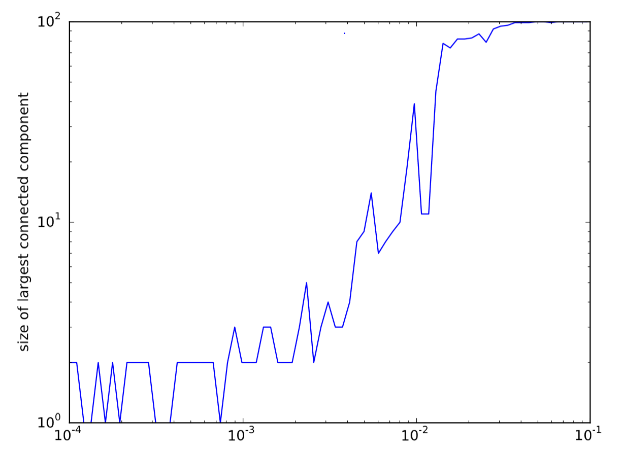
In this code, we measure the size of the largest connected component in an Erd˝os-R´enyi graph with connection probability $p$, while geometrically increasing $p$. The result shown in Fig. 17.1.2 indicates that a percolation transition happened at around $p = 10^{−2}$.

Figure 17.2.PNG — Figure $\PageIndex{2}$: Visual output of Code 17.4.

Giant components are a special name given to the largest connected components that appear above this percolation threshold (they are seen in the third and fourth panels of Fig. 17.1.1), because their sizes are on the same order of magnitude as the size of the whole network. Mathematically speaking, they are defined as the connected components whose size $s(n)$ has the following property

\[\lim_{n \rightarrow {\infty}} \frac{s(n)}{c}\ = \ c \ > \ 0, \label{(17.3)} \]

where $n$ is the number of nodes. This limit would go to zero for all other non-giant components, so at macroscopic scales, we can only see giant components in large networks.

Exercise $\PageIndex{1}$

Revise Code 17.4 so that you generate multiple random graphs for each $p$, and calculate the average size of the largest connected components. Then run the revised code for larger network sizes (say, 1,000) to obtain a smoother curve.

We can calculate the network percolation threshold for random graphs as follows. Let $q$ be the probability for a randomly selected node to not belong to the largest connected component (LCC) of a network. If $q < 1$, then there is a giant component in the network. In order for a randomly selected node to be disconnected from the LCC, all of its neighbors must be disconnected from the LCC too. Therefore, somewhat tautologically

\[q=q^{k}, \label{(17.4)} \]

where $k$ is the degree of the node in question. But in general, degree $k$ is not uniquely determined in a random network, so the right hand side should be rewritten as an expected value, as

\[q= \sum_{k=0}^{\infty}{P(k)q^{k}}, \label{(17.5)} \]

where $P(k)$ is the probability for the node to have degree $k$ (called the degree distribution; this will be discussed in more detail later). In an Erd˝os-R´enyi random graph, this probability can be calculated by the following binomial distribution

\[P(k) = \begin{cases} \binom{n-1}{k}p^{k}(1-p)^{n-1-k} & \text{ for } 0 \leq {k}\leq {n-1}, \label{(17.6)} \\ 0 & \text{ for } k \geq{n}, \end{cases} \]

because each node has $n−1$ potential neighbors and $k$ out of $n−1$ neighbors need to be connected to the node (and the rest need to be disconnected from it) in order for it to have degree $k$. By plugging Equation \ref{(17.6)} into Equation \ref{(17.5)}, we obtain
\[ \begin{align} q= \sum_{k=0}^{n-1}{\binom{n-1}{k}p^{k}(1-p)^{n-1-k}q^{k}} \label{(17.7)} \\ =\sum_{k=0}^{n-1}{\binom{n-1}{k}}(pq)^{k}(1-p)^{1-n-k} \label{(17.8)} \\ =(pq+1-p)^{n-1} \label{(17.9)} \\ =(1+p(q-1))^{n-1}. \label{(17.10)} \end{align} \]

We can rewrite this as

\[q=(1+ \frac{(k)(q-1)}{n}) ^{n-1}, \label{(17.11)} \]

because the average degree $(k)$ of an Erd˝os-R´enyi graph for a large $n$ is given by

\[(k) =np. \label{(17.12)} \]

Since $\lim_{n \rightarrow{\infty}} (1+x/n)^{n} =e^{x}$, Equation \ref{(17.11)} can be further simplified for large $n$ to

\[q= e^{(k) (q-1)}. \label{(17.13)} \]

Apparently, $q = 1$ satisfies this equation. If this equation also has another solution in $0 < q < 1$, then that means a giant component is possible in the network. Figure 17.1.3 shows the plots of $y = q $and $y = e^{(k)(q−1)}$ for $0 < q < 1$ for several values of $(k)$.

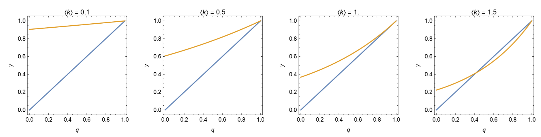
Figure 17.3.PNG — Figure $\PageIndex{3}$: Plots of $y = q$ and $y = e^{(k)(q−1)}$ for several values of $(k)$.

These plots indicate that if the derivative of the right hand side of Equation \ref{(17.13)} (i.e., the slope of the curve) at $q = 1$ is greater than 1, then the equation has a solution in $q < 1$. Therefore,

\[\frac{d}{dq}e^{(k)(q-1)}|_{q=1} =(k)e^{(k)(q-1)}\_{q=1} =(k) >1, \label{(17.14)} \]
i.e., if the average degree is greater than 1, then network percolation occurs.

A giant component is a connected component whose size is on the same order of magnitude as the size of the whole network. Network percolation is the appearance of such a giant component in a random graph, which occurs when the average node degree is above 1.

Exercise $\PageIndex{2}$

If Eq. (17.13) has a solution in $q < 1/n$, that means that all the nodes are essentially included in the giant component, and thus the network is made of a single connected component. Obtain the threshold of $(k)$ above which this occurs.