2.4: The Normal Distribution

There are many different types of distributions (shapes) of quantitative data. In section 1.5 we looked at different histograms and described the shapes of them as symmetric, skewed left, and skewed right. There is a special symmetric shaped distribution called the normal distribution. It is high in the middle and then goes down quickly and equally on both ends. It looks like a bell, so sometimes it is called a bell curve. One property of the normal distribution is that it is symmetric about the mean. Another property has to do with what percentage of the data falls within certain standard deviations of the mean. This property is defined as the empirical Rule.

The Empirical Rule: Given a data set that is approximately normally distributed:

Approximately 68% of the data is within one standard deviation of the mean.

Approximately 95% of the data is within two standard deviations of the mean.

Approximately 99.7% of the data is within three standard deviations of the mean.

To visualize these percentages, see the following figure.

Figure \(\PageIndex{1}\): Empirical Rule

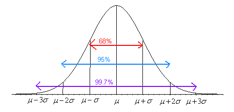
Note: The empirical rule is only true for approximately normal distributions.

Example \(\PageIndex{1}\): Using the Empirical Rule

Suppose that your class took a test and the mean score was 75% and the standard deviation was 5%. If the test scores follow an approximately normal distribution, answer the following questions:

1. What percentage of the students had scores between 65 and 85?
2. What percentage of the students had scores between 65 and 75?
3. What percentage of the students had scores between 70 and 80?
4. What percentage of the students had scores above 85?

To solve each of these, it would be helpful to draw the normal curve that follows this situation. The mean is 75, so the center is 75. The standard deviation is 5, so for each line above the mean add 5 and for each line below the mean subtract 5. The graph looks like the following:

Figure \(\PageIndex{2}\): Empirical Rule for Example \(\PageIndex{1}\)

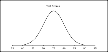
1. From the graph we can see that 95% of the students had scores between 65 and 85.
2. The scores of 65 to 75 are half of the area of the graph from 65 to 85. Because of symmetry, that means that the percentage for 65 to 85 is ½ of the 95%, which is 47.5%.
3. From the graph we can see that 68% of the students had scores between 70 and 80.
4. For this problem we need a bit of math. If you looked at the entire curve, you would say that 100% of all of the test scores fall under it. So because of symmetry 50% of the test scores fall in the area above the mean and 50% of the test scores fall in the area below the mean. We know from part b that the percentage from 65 to 75 is 47.5%. Because of symmetry, the percentage from 75 to 85 is also 47.5%. So the percentage above 85 is 50% - 47.5% = 2.5%.

When we look at Example \(\PageIndex{1}\), we realize that the numbers on the scale are not as important as how many standard deviations a number is from the mean. As an example, the number 80 is one standard deviation from the mean. The number 65 is 2 standard deviations from the mean. However, 80 is above the mean and 65 is below the mean. Suppose we wanted to know how many standard deviations the number 82 is from the mean. How would we do that? The other numbers were easier because they were a whole number of standard deviations from the mean. We need a way to quantify this. We will use a z-score (also known as a z-value or standardized score) to measure how many standard deviations a data value is from the mean. This is defined as:

z-score: \(z = \dfrac{x-\mu}{\sigma}\)

where \(x\) = data value (raw score)

\(z\) = standardized value (z-score or z-value)

\(\mu\) = population mean

\(\sigma\) = population standard deviation

Note: Remember that the z-score is always how many standard deviations a data value is from the mean of the distribution.

Suppose a data value has a z-score of 2.13. This tells us two things. First, it says that the data value is above the mean, since it is positive. Second, it tells us that you have to add more than two standard deviations to the mean to get to this value. Since most data (95%) is within two standard deviations, then anything outside this range would be considered a strange or unusual value. A z-score of 2.13 is outside this range so it is an unusual value. As another example, suppose a data value has a z-score of -1.34. This data value must be below the mean, since the z-score is negative, and you need to subtract more than one standard deviation from the mean to get to this value. Since this is within two standard deviations, it is an ordinary value.

An unusual value has a z-score < or a z-score > 2

A usual value has a z-score between and 2, that is \(-2 < z-score < 2\).

You may encounter standardized scores on reports for standardized tests or behavior tests as mentioned previously.

Example \(\PageIndex{2}\): Calculating Z-Scores

Suppose that your class took a test the mean score was 75% and the standard deviation was 5%. If test scores follow an approximately normal distribution, answer the following questions:

1. If a student earned 87 on the test, what is that student’s z-score and what does it mean?

\(\mu = 75\), \(\sigma = 5\), and \(x = 87\)

\(z = \dfrac{x-\mu}{\sigma}\)

\( = \dfrac{87-75}{5}\)

\(=2.40\)

This means that the score of 87 is more than two standard deviations above the mean, and so it is considered to be an unusual score.

2. If a student earned 73 on the test, what is that student’s z-score and what does it mean?

\(\mu = 75\), \(\sigma = 5\), and \(x = 73\)

\(z = \dfrac{x-\mu}{\sigma}\)

\( = \dfrac{73-75}{5}\)

\(=-0.40\)

This means that the score of 73 is less than one-half of a standard deviation below the mean. It is considered to be a usual or ordinary score.

3. If a student earned 54 on the test, what is that student’s z-score and what does it mean?

\(\mu = 75\), \(\sigma = 5\), and \(x = 54\)

\(z = \dfrac{x-\mu}{\sigma}\)

\( = \dfrac{54-75}{5}\)

\(=-4.20\)

The means that the score of 54 is more than four standard deviations below the mean, and so it is considered to be an unusual score.

4. If a student has a z-score of 1.43, what actual score did she get on the test?

\(\mu = 75\), \(\sigma = 5\), and \(z = 1.43\)

This problem involves a little bit of algebra. Do not worry, it is not that hard. Since you are now looking for x instead of z, rearrange the equation solving for x as follows:

\(z = \dfrac{x-\mu}{\sigma}\)

\(z \cdot \sigma= \dfrac{x-\mu}{\cancel{\sigma}} \cdot \cancel{\sigma}\)

\(z \sigma= x - \mu\)

\(z\sigma + \mu = x - \cancel{\mu} + \cancel{\mu}\)

\(x = z\sigma + \mu\)

Now, you can use this formula to find x when you are given z.

\(x = z\sigma + \mu \)

\(x = 1.43 \cdot 5 + 75 \)

\(x = 7.15 + 75 \)

\(x = 82.15 \)

Thus, the z-score of 1.43 corresponds to an actual test score of 82.15%.

5. If a student has a z-score of -2.34, what actual score did he get on the test?

\(\mu = 75\), \(\sigma = 5\), and \(z = -2.34\)

Use the formula for x from part d of this problem:

\(x = z\sigma + \mu \)

\(x = -2.34 \cdot 5 + 75 \)

\(x = -11.7 + 75 \)

\(x = 63.3 \)

Thus, the z-score of -2.34 corresponds to an actual test score of 63.3%.

The Five-Number Summary for a Normal Distribution

Looking at the Empirical Rule, 99.7% of all of the data is within three standard deviations of the mean. This means that an approximation for the minimum value in a normal distribution is the mean minus three times the standard deviation, and for the maximum is the mean plus three times the standard deviation. In a normal distribution, the mean and median are the same. Lastly, the first quartile can be approximated by subtracting 0.67448 times the standard deviation from the mean, and the third quartile can be approximated by adding 0.67448 times the standard deviation to the mean. All of these together give the five-number summary.

In mathematical notation, the five-number summary for the normal distribution with mean and standard deviation is as follows:

Five-Number Summary for a Normal Distribution

\(min = \mu - 3\sigma\)

\(Q_{1} = \mu - 0.67448\sigma\)

\(med = \mu \)

\(Q_{3} = \mu + 0.67448\sigma\)

\(max = \mu + 3\sigma\)

Example \(\PageIndex{3}\): Calculating the Five-Number Summary for a Normal Distribution

Suppose that your class took a test and the mean score was 75% and the standard deviation was 5%. If the test scores follow an approximately normal distribution, find the five-number summary.

The mean is \(\mu = 75 \%\) and the standard deviation is \(\sigma = 5 \%\). Thus, the five-number summary for this problem is:

\(min = 75 - 3(5) = 60 \%\)

\(Q_{1} = 75 - 0.67448(5)\approx 71.6 \%\)

\(med = 75 \% \)

\(Q_{3} = 75 + 0.67448(5)\approx 78.4 \%\)

\(max = 75 + 3(5) = 90 \%\)