11.5: Examples of Biological Cellular Automata Models

In this final section, I provide more examples of cellular automata models, with a particular emphasis on biological systems. Nearly all biological phenomena involve some kind of spatial extension, such as excitation patterns on neural or muscular tissue, cellular arrangements in an individual organism’s body, and population distribution at ecological levels. If a system has a spatial extension, nonlinear local interactions among its components may cause spontaneous pattern formation, i.e., self-organization of static or dynamic spatial patterns from initially uniform conditions. Such self-organizing dynamics are quite counter-intuitive, yet they play essential roles in the structure and function of biological systems.

In each of the following examples, I provide basic ideas of the state-transition rules and what kind of patterns can arise if some conditions are met. I assume Moore neighborhoods in these examples (unless noted otherwise), but the shape of the neighborhoods is not so critically important. Completed Python simulator codes are available from http://sourceforge.net/projects/pycx/files/, but you should try implementing your own simulator codes first.

Turing patterns

Animal skin patterns are a beautiful example of pattern formation in biological systems. To provide a theoretical basis of this intriguing phenomenon, British mathematician Alan Turing (who is best known for his fundamental work in theoretical computer science and for his code-breaking work during World War II) developed a family of models of spatio-temporal dynamics of chemical reaction and diffusion processes [44]. His original model was first written in a set of coupled ordinary differential equations on compartmentalized cellular structures, and then it was extended to partial differential equations (PDEs) in a continuous space. Later, a much simpler CA version of the same model was proposed by David Young [45]. We will discuss Young’s simpler model here.

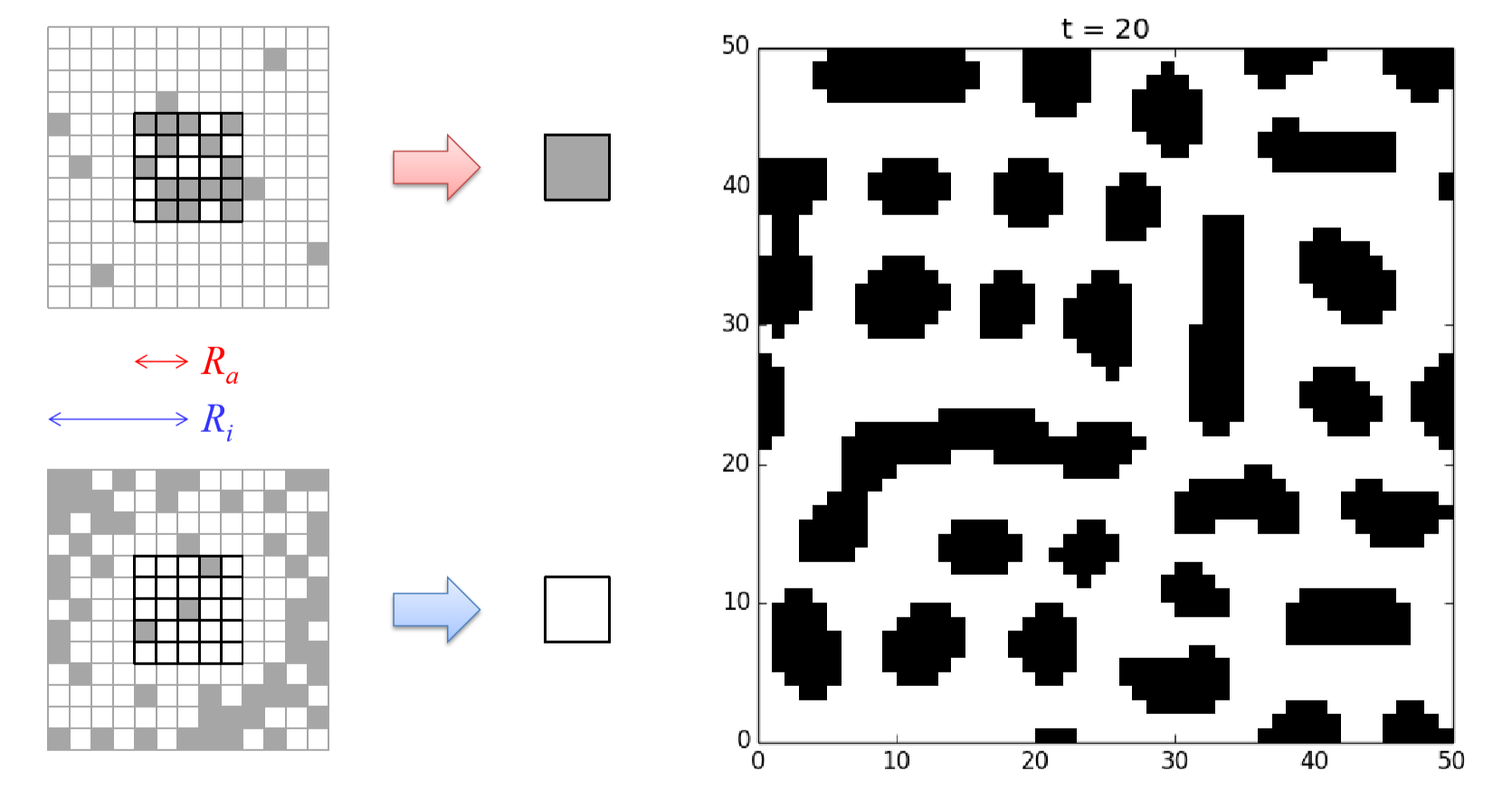
Assume a two-dimensional space made of cells where each cell can take either a passive (0) or active (1) state. A cell becomes activated if there are a sufficient number of active cells within its local neighborhood. However, other active cells outside this neighborhood try to suppress the activation of the focal cell with relatively weaker influences than those from the active cells in its close vicinity. These dynamics are called short-range activation and long-range inhibition. This model can be described mathematically as follows:

\[N_a= {x'| |x'| \leq R_a} \label{(11.4)} \]

\[N_i ={x'| |x'| \leq R_i}\label{(11.5)} \]

\[a_{t}(x)=w_{a} \sum_{x'\epsilon{N_{a}}}{s_{t}(x+x')} -w_{i} \sum_{x' \epsilon{N_{i}}}{s_{t}(x+x')}\label{(11.6)} \]

\[x_{t+1}(x) =\begin {cases} & 1 \qquad \text{if} \ a_{t}(x)>0, \\&0 \qquad \text{otherwise.} \end{cases} \label{(11.7)} \]

Here, \(R_a\) and \(R_i\) are the radii of neighborhoods for activation (\(N_a\)) and inhibition (\(N_i\)), respectively (\(R_{a} < R_{i})\), and \(w_a\) and \(w_i\) are the weights that represent their relative strengths. \(a_{t}(x)\) is the result of two neighborhood countings, which tells you whether the short-range activation wins ( \(a_{t}(x) > 0\) ) or the long-range inhibition wins \((a_{t}(x) \leq{0})\)at location \(x\). Figure 11.10 shows the schematic illustration of this state-transition function, as well as a sample simulation result you can get if you implement this model successfully.

Exercise \(\PageIndex{1}\):

Implement a CA model of the Turing pattern formation in Python. Then try the following:

• What happens if \(R_a\) and \(R_i\) are varied?
• What happens if \(w_a\) and \(w_i\) are varied?

Waves in excitable media

Neural and muscle tissues made of animal cells can generate and propagate electrophysiological signals. These cells can get excited in response to external stimuli coming from nearby cells, and they can generate action potential across their cell membranes that will be transmitted as a stimulus to other nearby cells. Once excited, the cell goes through a refractory period during which it doesn’t respond to any further stimuli. This causes the directionality of signal propagation and the formation of “traveling waves” on tissues.

Figure \(\PageIndex{1}\): Visual output of Code 11.5. Left: Initial configuration with \(p = 0.1\). Right: Final configuration after 20 time steps.

This kind of spatial dynamics, driven by propagation of states between adjacent cells that are physically touching each other, are called contact processes. This model and the following two are all examples of contact processes.

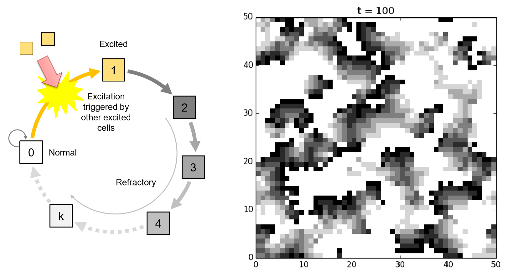
A stylized CA model of this excitable media can be developed as follows. Assume a two-dimensional space made of cells where each cell takes either a normal (0;quiescent), excited (1), or refractory (2, 3, ...\(k\)) state. A normal cell becomes excited stochastically with a probability determined by a function of the number of excited cells in its neighborhood. An excited cell becomes refractory (2) immediately, while a refractory cell remains refractory for a while (but its state keeps counting up) and then it comes back to normal after it reaches \(k\). Figure 11.5.2 shows the schematic illustration of this state-transition function, as well as a sample simulation result you can get if you implement this model successfully. These kinds of uncoordinated traveling waves of excitation (including spirals) are actually experimentally observable on the surface of a human heart under cardiac arrhythmia.

Exercise \(\PageIndex{2}\):

Implement a CA model of excitable media in Python. Then try the following:

Figure \(\PageIndex{2}\): CA model of excitable media. Left: Schematic illustration of the model’s state-transition function. Right: A sample simulation result.

• What happens if the excitation probability is changed?
• What happens if the length of the refractory period is changed?

Host-pathogen model

A spatially extended host-pathogen model, studied in theoretical biology and epidemiology, is a nice example to demonstrate the subtle relationship between these two antagonistic players. This model can also be viewed as a spatially extended version of the Lotka-Volterra (predator-prey) model, where each cell at a particular location represents either an empty space or an individual organism, instead of population densities that the variables in the Lotka-Volterra model represented.

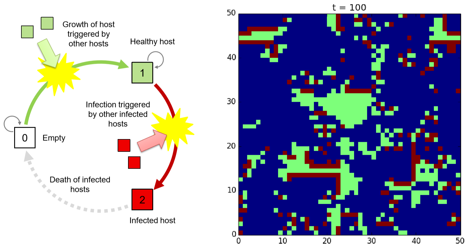
Assume a two-dimensional space filled with empty sites (0; quiescent) in which a small number of host organisms are initially populated. Some of them are “infected” by pathogens. A healthy host (1; also quiescent) without pathogens will grow into nearby empty sites stochastically. A healthy host may get infected by pathogens with a probability determined by a function of the number of infected hosts (2) in its neighborhood. An infected host will die immediately (or after some period of time). Figure 11.5.3 shows the schematic illustration of this state-transition function, as well as a sample simulation result you could get if you implement this model successfully. Note that this model is similar to the excitable media model discussed above, with the difference that the healthy host state (which corresponds to the excited state in the previous example) is quiescent and thus can remain in the space indefinitely.

The spatial patterns formed in this model are quite different from those in the previously discussed models. Turing patterns and waves in excitable media have clear characteristic length scales (i.e., size of spots or width of waves), but the dynamic patterns formed in the host-pathogen model lacks such characteristic length scales. You will see a number of dynamically forming patches of various sizes, from tiny ones to very large continents.

Figure \(\PageIndex{3}\): CA model of host-pathogen systems. Left: Schematic illustration of the model’s state-transition function. Right: A sample simulation result.

Exercise \(\PageIndex{3}\):

Implement a CA model of host-pathogen systems in Python. Then try the following:

• What happens if the infection probability is changed?
• In what conditions will both hosts and pathogens co-exist? In what conditions can hosts exterminate pathogens? In what conditions will both of them become extinct?
• Plot the populations of healthy/infected hosts over time, and see if there are any temporal patterns you can observe.

Epidemic/forest fire model

The final example, the epidemic model, is also about contact processes similar to the previous two examples. One difference is that this model focuses more on static spatial distributions of organisms and their influence on the propagation of an infectious disease within a single epidemic event. This model is also known as the “forest fire” model, so let’s use this analogy.

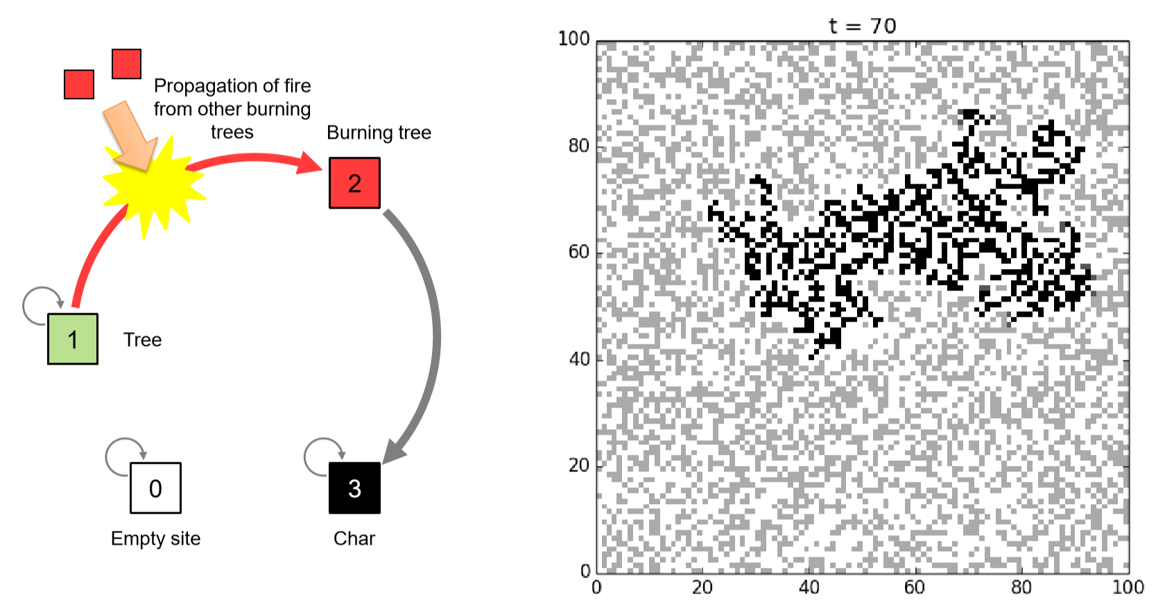
Assume there is a square-shaped geographical area, represented as a CA space, in which trees (1) are distributed with some given probability, \(p\). That is, \(p = 0\) means there are no trees in the space, whereas \(p = 1\) means trees are everywhere with no open space left in the area. Then, you set fire (2) to one of the trees in this forest to see if the fire you started eventually destroys the entire forest (don’t do this in real life!!). A tree will catch fire if there is at least one tree burning in its neighborhood, and the burning tree will be charred (3) completely after one time step.

Figure 11.5.4 shows the schematic illustration of this state-transition function, as well as a sample simulation result you could get if you implement this model successfully. Note that this model doesn’t have cyclic local dynamics; possible state transitions are always one way from a tree (1) to a burning tree (2) to being charred (3), which is different from the previous two examples. So the whole system eventually falls into a static final configuration with no further changes possible. But the total area burned in the final configuration greatly depends on the density of trees \(p\). If you start with a sufficiently large value of \(p\), you will see that a significant portion of the forest will be burned down eventually. This phenomenon is called percolation in statistical physics, which intuitively means that something found a way to go through a large portion of material from one side to the other.

Exercise \(\PageIndex{4}\):

Implement a CA model of epidemic/forest fire systems in Python. Then try the following:

• Compare the final results for different values of \(p\).
• Plot the total burned area as a function of \(p\).
• Plot the time until the fire stops spreading as a function of \(p\).

When you work on the above tasks, make sure to carry out multiple independent simulation runs for each value of \(p\) and average the results to obtain statistically

Figure \(\PageIndex{3}\): CA model of host-pathogen systems. Left: Schematic illustration of the model’s state-transition function. Right: A sample simulation result.

more reliable results. Such simulation methods based on random sampling are generally called Monte Carlo simulations. In Monte Carlo simulations, you conduct many replications of independent simulation runs for the same experimental settings, and measure the outcome variables from each run to obtain a statistical distribution of the measurements. Using this distribution (e.g., by calculating its average value) will help you enhance the accuracy and reliability of the experimental results.

If you have done the implementation and experiments correctly, you will probably see another case of phase transition in the exercise above. The system’s response shows a sharp transition at a critical value of p, above which percolation occurs but below which it doesn’t occur. Near this critical value, the system is very sensitive to minor perturbations, and a number of intriguing phenomena (such as the formation of self-similar fractal patterns) are found to take place at or near this transition point, which are called critical behaviors. Many complex systems, including biological and social ones, are considered to be utilizing such critical behaviors for their self-organizing and information processing purposes. For example, there is a conjecture that animal brains tend to dynamically maintain critical states in their neural dynamics in order to maximize their information processing capabilities. Such self-organized criticality in natural systems has been a fundamental research topic in complex systems science.