
13.3: Visualizing Two-Dimensional Scalar and Vector Field
- Page ID
- 7845

Plotting scalar and vector fields in Python is straightforward, as long as the space is two-dimensional. Here is an example of how to plot a 3-D surface plot:
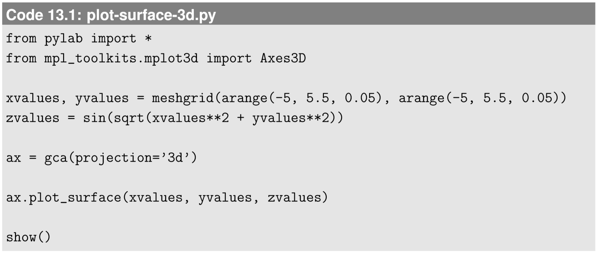
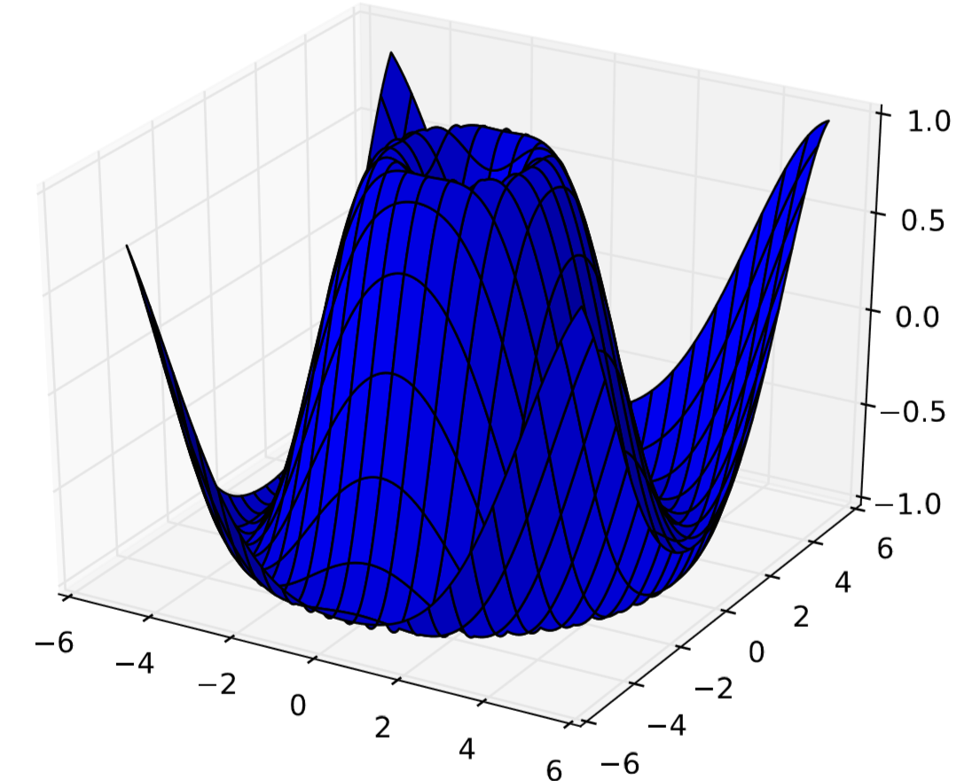
The scalar field \(f(x,y) = \sin{\sqrt{x^2 + y^2}}\) is given on the right hand side of the zvalues part. The result is shown in Fig. 13.3.1.
And here is how to draw a contour plot of the same scalar field:
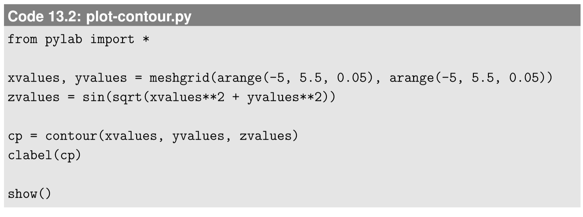
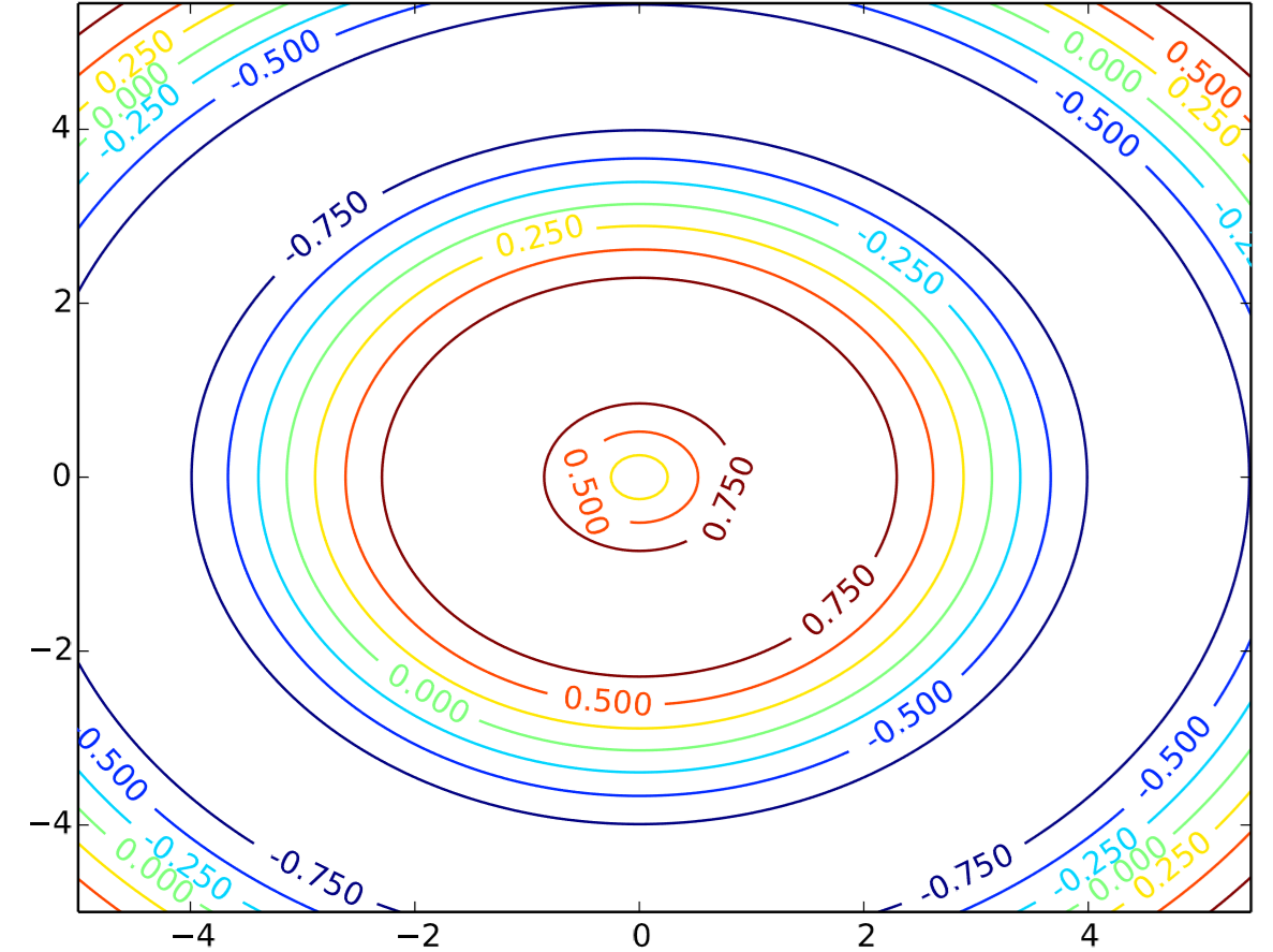
The clabel command is used here to add labels to the contours. The result is shown in Fig. 13.3.2.
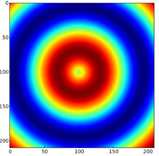
If you want more color, you can use imshow, which we already used for CA:

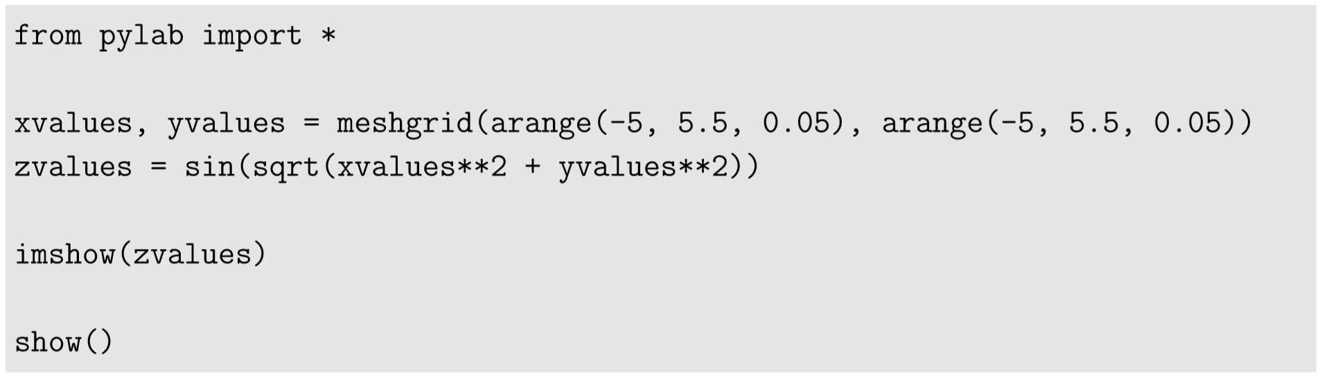
The result is shown in Fig. 13.3.3. Colorful!
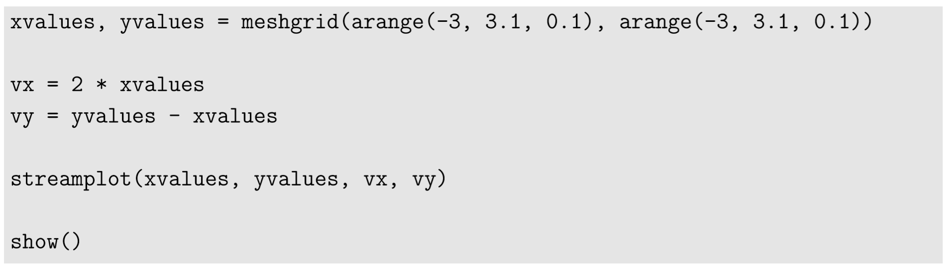
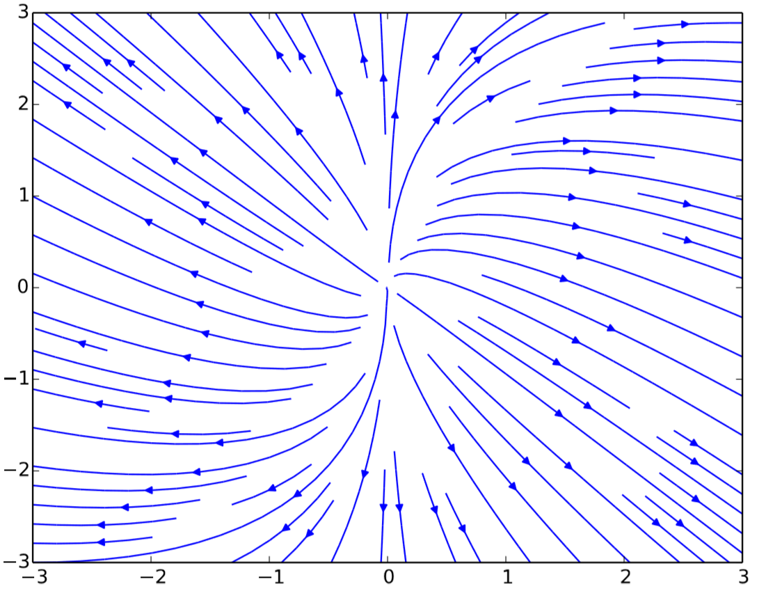
Finally, a two-dimensional vector field can be visualized using the streamplot function that we used in Section 7.2. Here is an example of the visualization of a vector field v = (vx,vy) = (2x,y−x), with the result shown in Fig. 13.3.4:

Plot the scalar field \(f(x,y) = \sin{(xy)}\) for \(−4 ≤ x,y ≤ 4\) using Python.
Plot the gradient field of f\((x,y) = \sin{(xy)}\) for \(−4 ≤ x,y ≤ 4\) using Python.
Plot the Laplacian of \(f(x,y) = \sin{(xy)}\) for \(−4 ≤ x,y ≤ 4\) using Python. Compare the result with the outputs of the exercises above.