1.4: The Lotka-Volterra Predator-Prey Model
- Page ID
- 93493

\(1.4\) The Lotka-Volterra predator-prey model
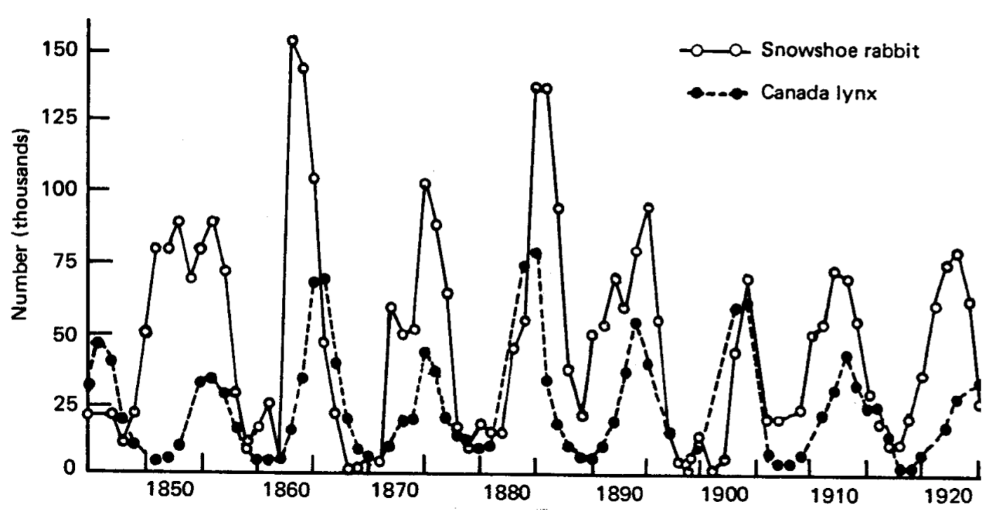
Pelt-trading records (Fig. 1.4) of the Hudson Bay company from over almost a century display a near-periodic oscillation in the number of trapped snowshoe hares and lynxes. With the reasonable assumption that the recorded number of trapped animals is proportional to the animal population, these records suggest that predator-prey populations-as typified by the hare and the lynx-can oscillate over time. Lotka and Volterra independently proposed in the 1920 s a mathematical model for the population dynamics of a predator and prey, and these Lotka-Volterra predator-prey equations have since become an iconic model of mathematical biology.
To develop these equations, suppose that a predator population feeds on a prey population. We assume that the number of prey grow exponentially in the absence of predators (there is unlimited food available to the prey), and that the number of predators decay exponentially in the absence of prey (predators must eat prey or starve). Contact between predators and prey increases the number of predators and decreases the number of prey.
Let \(U(t)\) and \(V(t)\) be the number of prey and predators at time \(t\). To develop a coupled differential equation model, we consider population sizes at time \(t+\Delta t\).
Exponential growth of prey in the absence of predators and exponential decay of predators in the absence of prey can be modeled by the usual linear terms. The coupling between prey and predator must be modeled with two additional parameters. We write the population sizes at time \(t+\Delta t\) as
\[\begin{aligned} &U(t+\Delta t)=U(t)+\alpha \Delta t U(t)-\gamma \Delta t U(t) V(t) \\[4pt] &V(t+\Delta t)=V(t)+e \gamma \Delta t U(t) V(t)-\beta \Delta t V(t) \end{aligned} \nonumber \]
The parameters \(\alpha\) and \(\beta\) are the average per capita birthrate of the prey and the deathrate of the predators, in the absence of the other species. The coupling terms model contact between predators and prey. The parameter \(\gamma\) is the fraction of prey caught per predator per unit time; the total number of prey caught by predators during time \(\Delta t\) is \(\gamma \Delta t U V\). The prey eaten is then converted into newborn predators (view this as a conversion of biomass), with conversion factor \(e\), so that the number of predators during time \(\Delta t\) increases by e\gamma \(\Delta t U V\).
Converting these equations into differential equations by letting \(\Delta t \rightarrow 0\), we obtain the well-known Lotka-Volterra predator-prey equations
\[\frac{d U}{d t}=\alpha U-\gamma U V, \quad \frac{d V}{d t}=e \gamma U V-\beta V \nonumber \]
Before analyzing the Lotka-Volterra equations, we first review fixed point and linear stability analysis applied to what is called an autonomous system of differential equations. For simplicity, we consider a system of only two differential equations of the form
\[\dot{x}=f(x, y), \quad \dot{y}=g(x, y), \nonumber \]
though our results can be generalized to larger systems. The system given by (1.4.2) is said to be autonomous since \(f\) and \(g\) do not depend explicitly on the independent variable \(t\). Fixed points of this system are determined by setting \(\dot{x}=\dot{y}=0\) and solving for \(x\) and \(y\). Suppose that one fixed point is \(\left(x_{*}, y_{*}\right)\). To determine its linear stability, we consider initial conditions for \((x, y)\) near the fixed point with small independent perturbations in both directions, i.e., \(x(0)=x_{*}+\epsilon(0), y(0)=\) \(y_{*}+\delta(0)\). If the initial perturbation grows in time, we say that the fixed point is unstable; if it decays, we say that the fixed point is stable. Accordingly, we let
\[x(t)=x_{*}+\epsilon(t), \quad y(t)=y_{*}+\delta(t), \nonumber \]
and substitute \((1.4.3)\) into \((1.4.2)\) to determine the time-dependence of \(\epsilon\) and \(\delta .\) Since \(x_{*}\) and \(y_{*}\) are constants, we have
\[\dot{\epsilon}=f\left(x_{*}+\epsilon, y_{*}+\delta\right), \quad \dot{\delta}=g\left(x_{*}+\epsilon, y_{*}+\delta\right) \nonumber \]
The linear stability analysis proceeds by assuming that the initial perturbations \(\epsilon(0)\) and \(\delta(0)\) are small enough to truncate the two-dimensional Taylor-series expansion of \(f\) and \(g\) about \(\epsilon=\delta=0\) to first-order in \(\epsilon\) and \(\delta\). Note that in general, the two-dimensional Taylor series of a function \(F(x, y)\) about the origin is given by
\[\begin{aligned} F(x, y)=F(0,0)+x F_{x}(0,0) &+y F_{y}(0,0) \\[4pt] &+\frac{1}{2}\left[x^{2} F_{x x}(0,0)+2 x y F_{x y}(0,0)+y^{2} F_{y y}(0,0)\right]+\ldots \end{aligned} \nonumber \]
where the terms in the expansion can be remembered by requiring that all of the partial derivatives of the series agree with that of \(F(x, y)\) at the origin. We now Taylor-series expand \(f\left(x_{*}+\epsilon, y_{*}+\delta\right)\) and \(g\left(x_{*}+\epsilon, y_{*}+\delta\right)\) about \((\epsilon, \delta)=(0,0)\). The constant terms vanish since \(\left(x_{*}, y_{*}\right)\) is a fixed point, and we neglect all terms with higher orders than \(\epsilon\) and \(\delta\). Therefore,
\[\dot{\epsilon}=\epsilon f_{x}\left(x_{*}, y_{*}\right)+\delta f_{y}\left(x_{*}, y_{*}\right), \quad \dot{\delta}=\epsilon g_{x}\left(x_{*}, y_{*}\right)+\delta g_{y}\left(x_{*}, y_{*}\right), \nonumber \]
which may be written in matrix form as
\[\frac{d}{d t}\left(\begin{array}{l} \epsilon \\[4pt] \delta \end{array}\right)=\left(\begin{array}{ll} f_{x}^{*} & f_{y}^{*} \\[4pt] g_{x}^{*} & g_{y}^{*} \end{array}\right)\left(\begin{array}{l} \epsilon \\[4pt] \delta \end{array}\right) \nonumber \]
where \(f_{x}^{*}=f_{x}\left(x_{*}, y_{*}\right)\), etc. Equation (1.4.6) is a system of linear ode’s, and its solution proceeds by assuming the form
\[\left(\begin{array}{l} \epsilon \\[4pt] \delta \end{array}\right)=e^{\lambda t} \mathbf{v} \nonumber \]
Upon substitution of \((1.4.7)\) into \((1.4.6)\), and canceling \(e^{\lambda t}\), we obtain the linear algebra eigenvalue problem
\[\mathrm{J}^{*} \mathbf{v}=\lambda \mathbf{v}, \text { with } \mathrm{J}^{*}=\left(\begin{array}{ll} f_{x}^{*} & f_{y}^{*} \\[4pt] g_{x}^{*} & g_{y}^{*} \end{array}\right) \nonumber \]
where \(\lambda\) is the eigenvalue, \(\mathbf{v}\) the corresponding eigenvector, and \(\mathrm{J}^{*}\) the Jacobian matrix evaluated at the fixed point. The eigenvalue is determined from the characteristic equation
\[\operatorname{det}\left(J^{*}-\lambda I\right)=0 \text {, } \nonumber \]
which for a two-by-two Jacobian matrix results in a quadratic equation for \(\lambda\). From the form of the solution \((1.4.7)\), the fixed point is stable if for all eigenvalues \(\lambda\), \(\operatorname{Re}\{\lambda\}<0\), and unstable if for at least one \(\lambda, \operatorname{Re}\{\lambda\}>0 .\) Here \(\operatorname{Re}\{\lambda\}\) means the real part of the (possibly) complex eigenvalue \(\lambda\). We now reconsider the Lotka-Volterra equations. Fixed point solutions are found by solving \(\dot{U}=\dot{V}=0\), and we have from (1.4.1)
\[U(\alpha-\gamma V)=0, \quad V(e \gamma U-\beta)=0 \nonumber \]
Evidently the only two possible solutions are
\[\left(U_{*}, V_{*}\right)=(0,0) \text { or }\left(\frac{\beta}{e \gamma}, \frac{\alpha}{\gamma}\right) . \nonumber \]
The trivial fixed point \((0,0)\) is unstable since the prey population grows exponentially if it is initially small. To determine the stability of the second fixed point, we write the Lotka-Volterra equation in the form
\[\frac{d U}{d t}=F(U, V), \quad \frac{d V}{d t}=G(U, V) \nonumber \]
with
\[F(U, V)=\alpha U-\gamma U V, \quad G(U, V)=e \gamma U V-\beta V \nonumber \]
The partial derivatives are then computed to be
\[\begin{array}{ll} F_{U}=\alpha-\gamma V, & F_{V}=-\gamma U \\[4pt] G_{U}=e \gamma V, & G_{V}=e \gamma U-\beta . \end{array} \nonumber \]
The Jacobian at the fixed point \(\left(U_{*}, V_{*}\right)=(\beta / e \gamma, \alpha / \gamma)\) is
\[J^{*}=\left(\begin{array}{cc} 0 & -\beta / e \\[4pt] e \alpha & 0 \end{array}\right) \nonumber \]
and
\[\begin{aligned} \operatorname{det}\left(\mathrm{J}^{*}-\lambda \mathrm{I}\right) &=\left|\begin{array}{cc} -\lambda & -\beta / e \\[4pt] e \alpha & -\lambda \end{array}\right| \\[4pt] &=\lambda^{2}+\alpha \beta \\[4pt] &=0 \end{aligned} \nonumber \]
has the solutions \(\lambda_{\pm}=\pm i \sqrt{\alpha \beta}\), which are pure imaginary. When the eigenvalues of the two-by-two Jacobian are pure imaginary, the fixed point is called a center and the perturbation neither grows nor decays, but oscillates. Here, the angular frequency of oscillation is \(\omega=\sqrt{\alpha \beta}\), and the period of the oscillation is \(2 \pi / \omega\).
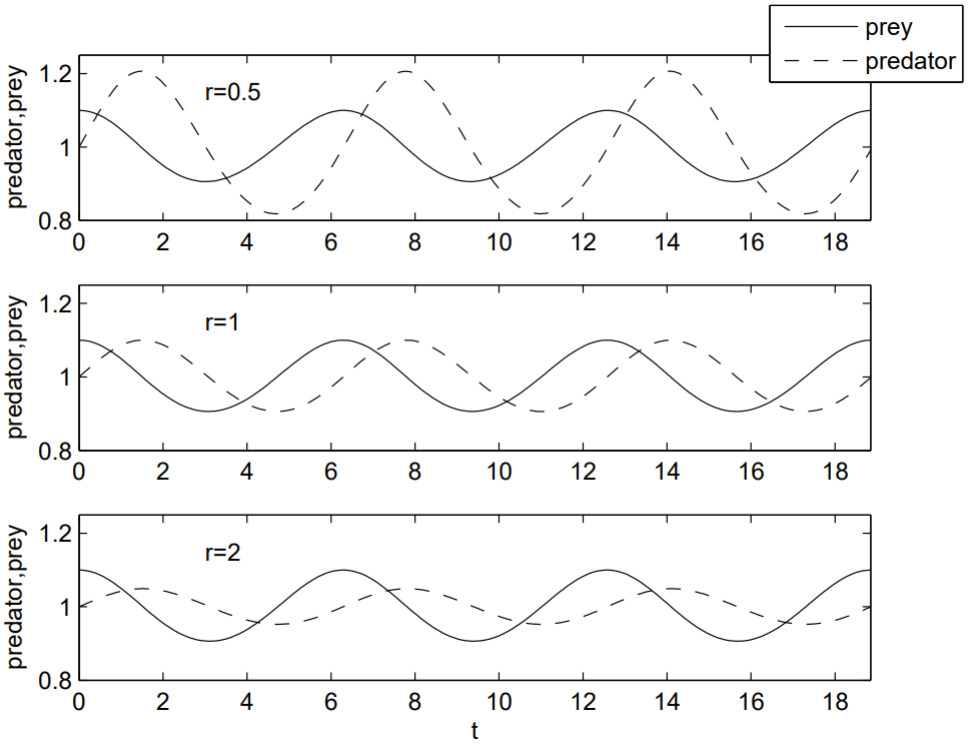
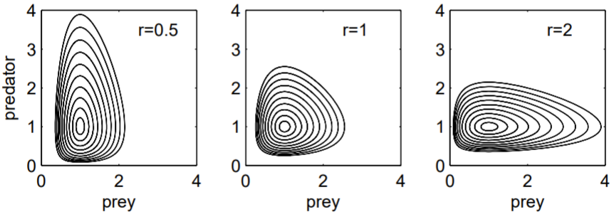
We plot \(U\) and \(V\) versus \(t\) (time series plot), and \(V\) versus \(U\) (phase portraits) to see how the solutions behave. For a nonlinear system of equations such as (1.4.1), a numerical solution is required.
The Lotka-Volterra equations has four free parameters \(\alpha, \beta, \gamma\) and \(e\). The relevant units here are time, the number of prey, and the number of predators. The Buckingham \(\mathrm{Pi}\) Theorem predicts that nondimensionalizing the equations can reduce the number of free parameters by three to a manageable single dimensionless grouping of parameters. We choose to nondimensionalize time using the angular frequency of oscillation and the number of prey and predators using their fixed point values. With carets denoting the dimensionless variables, we let
\[\hat{t}=\sqrt{\alpha \beta} t, \quad \hat{U}=U / U_{*}=\frac{e \gamma}{\beta} U, \quad \hat{V}=V / V_{*}=\frac{\gamma}{\alpha} V \nonumber \]
Substitution of (1.4.16) into the Lotka-Volterra equations (1.4.1) results in the dimensionless equations
\[\frac{d \hat{U}}{d \hat{t}}=r(\hat{U}-\hat{U} \hat{V}), \quad \frac{d \hat{V}}{d \hat{t}}=\frac{1}{r}(\hat{U} \hat{V}-\hat{V}) \nonumber \]
with single dimensionless grouping \(r=\sqrt{\alpha / \beta} .\) Specification of \(r\) together with initial conditions completely determines the solution. It should be noted here that the long-time solution of the Lotka-Volterra equations depends on the initial conditions. This asymptotic dependence on the initial conditions is usually considered a flaw of the model.
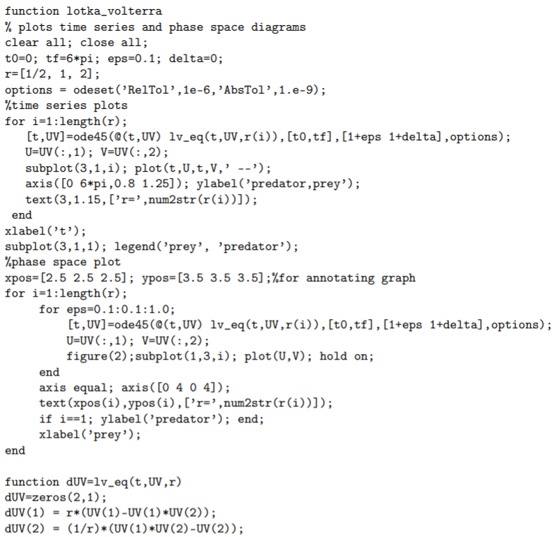
A numerical solution uses MATLAB’s ode45.m built-in function to integrate the differential equations. The code below produces Fig. 1.5. Notice how the predator population lags the prey population: an increase in prey numbers results in a delayed increase in predator numbers as the predators eat more prey. The phase portraits clearly show the periodicity of the oscillation. Note that the curves move counterclockwise: prey numbers increase when predator numbers are minimal, and prey numbers decrease when predator numbers are maximal.