43.3: Variability and MAD

Last updated
Save as PDF

Page ID: 40876

\( \newcommand{\vecs}[1]{\overset { \scriptstyle \rightharpoonup} {\mathbf{#1}} } \) \( \newcommand{\vecd}[1]{\overset{-\!-\!\rightharpoonup}{\vphantom{a}\smash {#1}}} \)\(\newcommand{\id}{\mathrm{id}}\) \( \newcommand{\Span}{\mathrm{span}}\) \( \newcommand{\kernel}{\mathrm{null}\,}\) \( \newcommand{\range}{\mathrm{range}\,}\) \( \newcommand{\RealPart}{\mathrm{Re}}\) \( \newcommand{\ImaginaryPart}{\mathrm{Im}}\) \( \newcommand{\Argument}{\mathrm{Arg}}\) \( \newcommand{\norm}[1]{\| #1 \|}\) \( \newcommand{\inner}[2]{\langle #1, #2 \rangle}\) \( \newcommand{\Span}{\mathrm{span}}\) \(\newcommand{\id}{\mathrm{id}}\) \( \newcommand{\Span}{\mathrm{span}}\) \( \newcommand{\kernel}{\mathrm{null}\,}\) \( \newcommand{\range}{\mathrm{range}\,}\) \( \newcommand{\RealPart}{\mathrm{Re}}\) \( \newcommand{\ImaginaryPart}{\mathrm{Im}}\) \( \newcommand{\Argument}{\mathrm{Arg}}\) \( \newcommand{\norm}[1]{\| #1 \|}\) \( \newcommand{\inner}[2]{\langle #1, #2 \rangle}\) \( \newcommand{\Span}{\mathrm{span}}\)\(\newcommand{\AA}{\unicode[.8,0]{x212B}}\)

Lesson

Let's study distances between data points and the mean and see what they tell us.

Exercise \(\PageIndex{1}\): Shooting Hoops (Part 1)

Elena, Jada, and Lin enjoy playing basketball during recess. Lately, they have been practicing free throws. They record the number of baskets they make out of 10 attempts. Here are their data sets for 12 school days.

Elena

\(4\qquad 5\qquad 1\qquad 6\qquad 9\qquad 7\qquad 2\qquad 8\qquad 3\qquad 3\qquad 5\qquad 7\)

Jada

\(2\qquad 4\qquad 5\qquad 4\qquad 6\qquad 6\qquad 4\qquad 7\qquad 3\qquad 4\qquad 8\qquad 7\)

Lin

\(3\qquad 6\qquad 6\qquad 4\qquad 5\qquad 5\qquad 3\qquad 5\qquad 4\qquad 6\qquad 6\qquad 7\)

Calculate the mean number of baskets each player made, and compare the means. What do you notice?
What do the means tell us in this context?

Exercise \(\PageIndex{2}\): Shooting Hoops (Part 2)

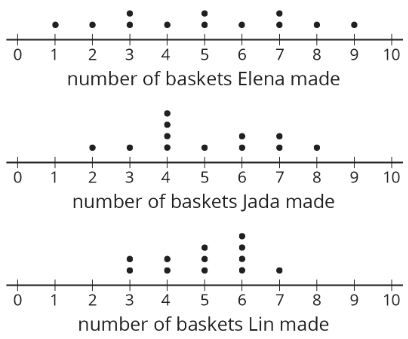
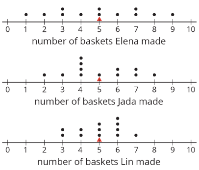
Here are the dot plots showing the number of baskets Elena, Jada, and Lin each made over 12 school days.

On each dot plot, mark the location of the mean with a triangle (\(\Delta\)). Then, contrast the dot plot distributions. Write 2–3 sentences to describe the shape and spread of each distribution.

Figure \(\PageIndex{1}\): Three dot plots, number of baskets made, 0 to 10 by ones. First plot, Elena, beginning at 1 number of dots above each increment is 1, 1, 2, 1, 2, 1, 2, 1, 1. Second plot, Jada, beginning at 2 the number of dots above each increment is 1, 1, 4, 1, 2, 2, 1. Third plot, Lin, beginning at 3 the number of dots above each increment is 2, 2, 3, 4, 1.

Discuss the following questions with your group. Explain your reasoning.
1. Would you say that all three students play equally well?
2. Would you say that all three students play equally consistently?
3. If you could choose one player to be on your basketball team based on their records, who would you choose?

Exercise \(\PageIndex{3}\): Shooting Hoops (Part 3)

The tables show Elena, Jada, and Lin’s basketball data from an earlier activity. Recall that the mean of Elena’s data, as well as that of Jada and Lin’s data, was 5.

Record the distance between each of Elena’s scores and the mean.

Table \(\PageIndex{1}\)
Elena	\(4\)	\(5\)	\(1\)	\(6\)	\(9\)	\(7\)	\(2\)	\(8\)	\(3\)	\(3\)	\(5\)	\(7\)
distance from \(5\)	\(1\)			\(1\)

Now find the average of the distances in the table. Show your reasoning and round your answer to the nearest tenth.

This value is the mean absolute deviation (MAD) of Elena’s data.

Elena’s MAD: ________

Find the mean absolute deviation of Jada’s data. Round it to the nearest tenth.

Table \(\PageIndex{2}\)
Jada	\(2\)	\(4\)	\(5\)	\(4\)	\(6\)	\(6\)	\(4\)	\(7\)	\(3\)	\(4\)	\(8\)	\(7\)
distance from \(5\)

Jada’s MAD: _________

Find the mean absolute deviation of Lin’s data. Round it to the nearest tenth.

Table \(\PageIndex{3}\)
Lin	\(3\)	\(6\)	\(6\)	\(4\)	\(5\)	\(5\)	\(3\)	\(5\)	\(4\)	\(6\)	\(6\)	\(7\)
distance from \(5\)

Lin’s MAD: _________

Compare the MADs and dot plots of the three students’ data. Do you see a relationship between each student’s MAD and the distribution on her dot plot? Explain your reasoning.

Figure \(\PageIndex{2}\): Three dot plots, number of baskets made, 0 to 10 by ones. First plot, Elena, beginning at 1 number of dots above each increment is 1, 1, 2, 1, 2, 1, 2, 1, 1, triangle at 5. Second plot, Jada, beginning at 2 the number of dots above each increment is 1, 1, 4, 1, 2, 2, 1, triangle at 5. Third plot, Lin, beginning at 3 the number of dots above each increment is 2, 2, 3, 4, 1, triangle at 5.

Are you ready for more?

Invent another data set that also has a mean of 5 but has a MAD greater than 2. Remember, the values in the data set must be whole numbers from 0 to 10.

Exercise \(\PageIndex{4}\): Game of 22

Your teacher will give your group a deck of cards. Shuffle the cards, and put the deck face down on the playing surface.

To play: Draw 3 cards and add up the values. An ace is a 1. A jack, queen, and king are each worth 10. Cards 2–10 are each worth their face value. If your sum is anything other than 22 (either above or below 22), say: “My sum deviated from 22 by ____ ,” or “My sum was off from 22 by ____ .”
To keep score: Record each sum and each distance from 22 in the table. After five rounds, calculate the average of the distances. The player with the lowest average distance from 22 wins the game.

Table \(\PageIndex{4}\)
player A	round 1	round 2	round 3	round 4	round 5
sum of cards
distance from 22

Average distance from 22: ____________

Table \(\PageIndex{5}\)
player B	round 1	round 2	round 3	round 4	round 5
sum of cards
distance from 22

Average distance from 22: ____________

Table \(\PageIndex{6}\)
player C	round 1	round 2	round 3	round 4	round 5
sum of cards
distance from 22

Average distance from 22: ____________

Whose average distance from 22 is the smallest? Who won the game?

Summary

We use the mean of a data set as a measure of center of its distribution, but two data sets with the same mean could have very different distributions.

This dot plot shows the weights, in grams, of 22 cookies.

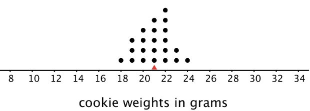
Figure \(\PageIndex{3}\): A dot plot for “cookie weights in grams.” The numbers 8 through 34, in increments of 2, are indicated. A triangle is indicated at 21 grams. The data are as follows: 18 grams, 1 dot; 19 grams, 3 dots; 20 grams, 4 dots; 21 grams, 5 dots; 22 grams, 6 dots; 23 grams, 2 dots, 24 grams, 1 dot.

The mean weight is 21 grams. All the weights are within 3 grams of the mean, and most of them are even closer. These cookies are all fairly close in weight.

This dot plot shows the weights, in grams, of a different set of 30 cookies.

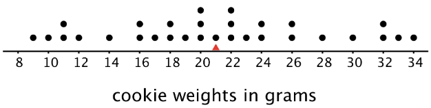
Figure \(\PageIndex{4}\): A dot plot for “cookie weights in grams.” The numbers 8 through 34, in increments of 2, are indicated. A triangle is indicated at 21 grams. The data are as follows: 9 grams, 1 dot; 10 grams, 1 dot; 11 grams, 2 dots; 12 grams, 1 dot; 14 grams, 1 dot; 16 grams, 2 dots; 17 grams, 1 dot; 18 grams, 2 dots; 19 grams, 1 dot; 20 grams, 3 dots; 21 grams, 1 dot; 22 grams, 3 dots; 23 grams, 1 dot; 24 grams, 2 dots; 26 grams, 2 dots; 28 grams, 1 dot; 30 grams, 1 dot; 32 grams, 2 dots; 33 grams, 1 dot; 34 grams, 1 dot.

The mean weight for this set of cookies is also 21 grams, but some cookies are half that weight and others are one-and-a-half times that weight. There is a lot more variability in the weight.

There is a number we can use to describe how far away, or how spread out, data points generally are from the mean. This measure of spread is called the mean absolute deviation (MAD).

Here the MAD tells us how far cookie weights typically are from 21 grams. To find the MAD, we find the distance between each data value and the mean, and then calculate the mean of those distances.

For instance, the point that represents 18 grams is 3 units away from the mean of 21 grams. We can find the distance between each point and the mean of 21 grams and organize the distances into a table, as shown.

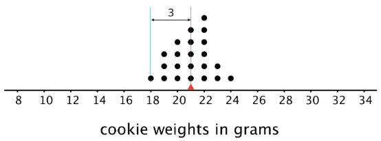
Figure \(\PageIndex{5}\): A dot plot for “cookie weights in grams.” The numbers 8 through 34, in increments of 2, are indicated. A triangle is indicated at 21 grams. There are two perpendicular lines drawn, one at 18 grams and the other at 21 grams. A horizontal line between the two lines is labeled 3. The data are as follows: 18 grams, 1 dot; 19 grams, 3 dots; 20 grams, 4 dots; 21 grams, 5 dots; 22 grams, 6 dots; 23 grams, 2 dots, 24 grams, 1 dot.

Table \(\PageIndex{7}\)
weight in grams	\(18\)	\(19\)	\(19\)	\(19\)	\(20\)	\(20\)	\(20\)	\(20\)	\(21\)	\(21\)	\(21\)	\(21\)	\(21\)	\(22\)	\(22\)	\(22\)	\(22\)	\(22\)	\(22\)	\(23\)	\(23\)	\(24\)
distance from mean	\(3\)	\(2\)	\(2\)	\(2\)	\(1\)	\(1\)	\(1\)	\(1\)	\(0\)	\(0\)	\(0\)	\(0\)	\(0\)	\(1\)	\(1\)	\(1\)	\(1\)	\(1\)	\(1\)	\(2\)	\(2\)	\(3\)

The values in the first row of the table are the cookie weights for the first set of cookies. Their mean, 21 grams, is the mean of the cookie weights.

The values in the second row of the table are the distances between the values in the first row and 21. The mean of these distances is the MAD of the cookie weights.

What can we learn from the averages of these distances once they are calculated?

In the first set of cookies, the distances are all between 0 and 3. The MAD is 1.2 grams, which tells us that the cookie weights are typically within 1.2 grams of 21 grams. We could say that a typical cookie weighs between 19.8 and 22.2 grams.
In the second set of cookies, the distances are all between 0 and 13. The MAD is 5.6 grams, which tells us that the cookie weights are typically within 5.6 grams of 21 grams. We could say a typical cookie weighs between 15.4 and 26.6 grams.

The MAD is also called a measure of the variability of the distribution. In these examples, it is easy to see that a higher MAD suggests a distribution that is more spread out, showing more variability.

Glossary Entries

Definition: Average

The average is another name for the mean of a data set.

For the data set 3, 5, 6, 8, 11, 12, the average is 7.5.

\(3+5+6+8+11+12=45\)

\(45\div 6=7.5\)

Definition: Mean

The mean is one way to measure the center of a data set. We can think of it as a balance point. For example, for the data set 7, 9, 12, 13, 14, the mean is 11.

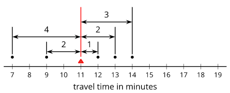
To find the mean, add up all the numbers in the data set. Then, divide by how many numbers there are. \(7+9+12+13+14=55\) and \(55\div 5=11\).

Definition: Mean Absolute Deviation (MAD)

The mean absolute deviation is one way to measure how spread out a data set is. Sometimes we call this the MAD. For example, for the data set 7, 9, 12, 13, 14, the MAD is 2.4. This tells us that these travel times are typically 2.4 minutes away from the mean, which is 11.

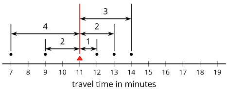
To find the MAD, add up the distance between each data point and the mean. Then, divide by how many numbers there are.

\(4+2+1+2+3=12\) and \(12\div 5=2.4\)

Definition: Measure of Center

A measure of center is a value that seems typical for a data distribution.

Mean and median are both measures of center.

Practice

Exercise \(\PageIndex{5}\)

Han recorded the number of pages that he read each day for five days. The dot plot shows his data.

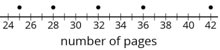
Is 30 pages a good estimate of the mean number of pages that Han read each day? Explain your reasoning.
Find the mean number of pages that Han read during the five days. Draw a triangle to mark the mean on the dot plot.

Use the dot plot and the mean to complete the table.

Table \(\PageIndex{8}\)
number of pages	distance from mean	left or right of mean
\(25\)		left
\(28\)
\(32\)
\(36\)
\(42\)

Calculate the mean absolute deviation (MAD) of the data. Explain or show your reasoning.

Exercise \(\PageIndex{6}\)

Ten sixth-grade students recorded the amounts of time each took to travel to school. The dot plot shows their travel times.

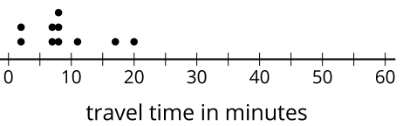
The mean travel time for these students is approximately 9 minutes. The MAD is approximately 4.2 minutes.

Which number of minutes—9 or 4.2—is a typical amount of time for the ten sixth-grade students to travel to school? Explain your reasoning.
Based on the mean and MAD, Jada believes that travel times between 5 and 13 minutes are common for this group. Do you agree? Explain your reasoning.
A different group of ten sixth-grade students also recorded their travel times to school. Their mean travel time was also 9 minutes, but the MAD was about 7 minutes. What could the dot plot of this second data set be? Describe or draw how it might look.

Exercise \(\PageIndex{7}\)

In an archery competition, scores for each round are calculated by averaging the distance of 3 arrows from the center of the target.

An archer has a mean distance of 1.6 inches and a MAD distance of 1.3 inches in the first round. In the second round, the archer's arrows are farther from the center but are more consistent. What values for the mean and MAD would fit this description for the second round? Explain your reasoning.