
3.E: The Integral (Exercises)
- Page ID
- 80592

3.1 Exercises
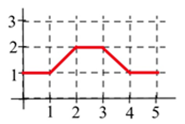
Let \(A(x)\) represent the area bounded by the graph and the horizontal axis and vertical lines at \(t=0\) and \(t=x\) for the graph shown. Evaluate \(A(x)\) for \(x =\) 1, 2, 3, 4, and 5.
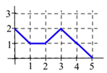
Let \(B(x)\) represent the area bounded by the graph and the horizontal axis and vertical lines at \(t=0\) and \(t=x\) for the graph shown. Evaluate \(B(x)\) for \(x =\) 1, 2, 3, 4, and 5.
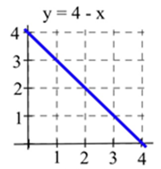
Let \(C(x)\) represent the area bounded by the graph and the horizontal axis and vertical lines at \(t=0\) and \(t=x\) for the graph shown. Evaluate \(C(x)\) for \(x =\) 1, 2, and 3 and find a formula for \(C(x)\).
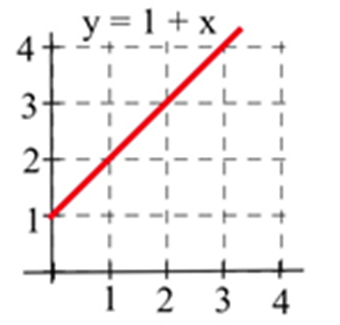
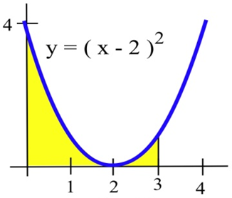
Let \(A(x)\) represent the area bounded by the graph and the horizontal axis and vertical lines at \(t=0\) and \(t=x\) for the graph shown. Evaluate \(A(x)\) for \(x =\) 1, 2, and 3 and find a formula for \(A(x)\).
A car had the velocity shown in the graph to the right.
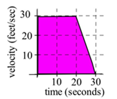
A car had the velocity shown in the graph to the right. How far did the car travel from \(t= 0\) to \(t = 30\) seconds?
A car had the velocity shown below.
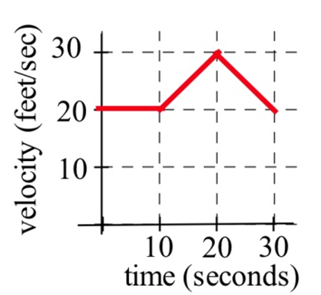
How afar did the car travel from \(t = 0\) to \(t = 30\) seconds?
The velocities of two cars are shown in the graph.
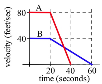
(a) From the time the brakes were applied, how many seconds did it take each car to stop?
(b) From the time the brakes were applied, which car traveled farther until it came to a complete stop?
You and a friend start off at noon and walk in the same direction along the same path at the rates shown.
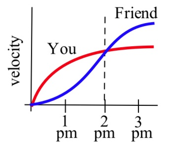
(a) Who is walking faster at 2 pm? Who is ahead at 2 pm?
(b) Who is walking faster at 3 pm? Who is ahead at 3 pm?
(c) When will you and your friend be together? (Answer in words.)
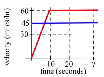
Police chase: A speeder traveling 45 miles per hour (in a 25 mph zone) passes a stopped police car which immediately takes off after the speeder. If the police car speeds up steadily to 60 miles/hour in 20 seconds and then travels at a steady 60 miles/hour, how long and how far before the police car catches the speeder who continued traveling at 45 miles/hour?
Water is flowing into a tub. The table shows the rate at which the water flows, in gallons per minute. The tub is initially empty.
|
\(t\), in minutes |
0 |
1 |
2 |
3 |
4 |
5 |
6 |
7 |
8 |
9 |
10 |
|
Flow rate, in gal/min |
0.5 |
1.0 |
1.2 |
1.4 |
1.7 |
2.0 |
2.3 |
1.8 |
0.7 |
0.5 |
0.2 |
Use the table to estimate how much water is in the tub after
a. five minutes
b. ten minutes
The table shows the speedometer readings for a short car trip.
|
\(t\), in minutes |
0 |
5 |
10 |
15 |
20 |
|
Speed, in mph |
0 |
30 |
40 |
65 |
40 |
a. Use the table to estimate how far the car traveled over the twenty minutes shown.
b. How accurate would you expect your estimate to be?
The table shows values of \(f(t)\). Use the table to estimate \(\int^{40}_0 f(t) dt\).
|
\(t\) |
0 |
10 |
20 |
30 |
40 |
|
\(f(t)\) |
17 |
22 |
18 |
11 |
35 |
The table shows values of \(g(x)\).
|
\(x\) |
0 |
1 |
2 |
3 |
4 |
5 |
6 |
|
\(g(x)\) |
140 |
142 |
144 |
152 |
154 |
165 |
200 |
Use the table to estimate
| a. \(\int^3_0 g(x) dx\) | b \(\int^6_3 g(x) dx\) | c. \(\int^6_0 g(x) dx\) |
What are the units for the "area" of a rectangle with the given base and height units?
| Base units | Height units | "Area" units |
|
miles per second |
seconds |
|
|
hours |
dollars per hour |
|
|
square feet |
feet |
|
|
kilowatts |
hours |
|
|
houses |
people per house |
|
|
meals |
meals |
In problems 15 – 17, represent the area of each bounded region as a definite integral, and use geometry to determine the value of the definite integral.
15. The region bounded by \(y = 2x \), the \(x\)–axis, the line \(x = 1\), and \(x = 3\).
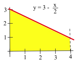
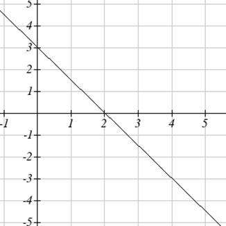
16. The region bounded by \(y = 4 – 2x \), the \(x\)–axis, and the \(y\)–axis.
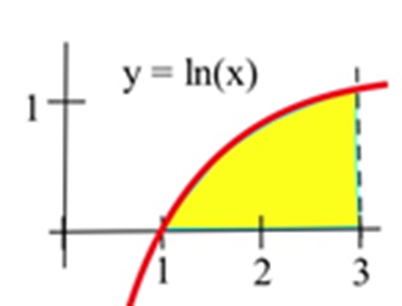
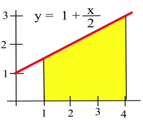
17. The shaded region in the graph to the right.
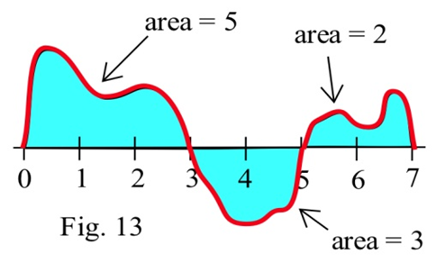
Using the graph of \(f\) shown and the given areas of several regions, evaluate:
(a) \(\int^3_0 f(x) dx\)
(b) \(\int^5_3 f(x) dx\)
(c) \(\int^7_5 f(x) dx\)
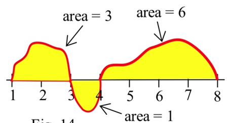
Using the graph of \(f\) shown and the given areas of several regions, evaluate:
(a) \(\int^3_1 g(x) dx\)
(b) \(\int^4_3 g(x) dx\)
(c) \(\int^8_4 g(x) dx\)
(d) \(\int^8_1 g(x) dx\)
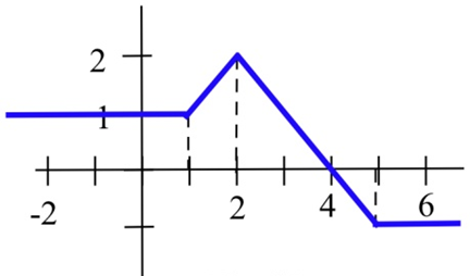
Use the graph to evaluate:
(a) \(\int^1_{-2} h(x) dx\)
(b) \(\int^6_4 h(x) dx\)
(c) \(\int^6_{-2} h(x) dx\)
(d) \(\int^4_{-2} h(x) dx\)
Your velocity along a straight road is shown to the right. How far did you travel in 8 minutes?
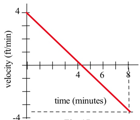
Your velocity along a straight road is shown below. How many feet did you walk in 8 minutes?
In problems 23 - 26, the units are given for \(x\) and for \(f(x)\). Give the units of \(\int^b_a f(x) dx\).
23. \(x\) is time in "seconds", and \(f(x)\) is velocity in "meters per second."
24. \(x\) is time in "hours", and \(f(x)\) is a flow rate in "gallons per hour."
25. \(x\) is a position in "feet", and \(f(x)\) is an area in "square feet."
26. \(x\) is a position in "inches", and \(f(x)\) is a density in "pounds per inch."
In problems 27 – 31, represent the area with a definite integral and use technology to find the approximate answer.
27. The region bounded by \(y = x^3\), the \(x\)–axis, the line \(x = 1\), and \(x = 5\).
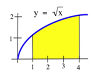
28. The region bounded by \(y = \sqrt{x}\), the \(x\)–axis, and the line \(x = 9\).
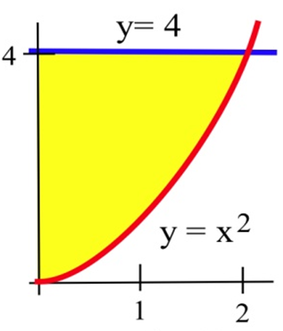
29. The shaded region shown to the right.
30. The shaded region below.
31. Consider the definite integral \(\int^3_0 (3+x) dx\).
(a) Using six rectangles, find the left-hand Riemann sum for this definite integral.
(b) Using six rectangles, find the right-hand Riemann sum for this definite integral.
(c) Using geometry, find the exact value of this definite integral.
Consider the definite integral \(\int^2_0 x^3 dx\).
(a) Using four rectangles, find the left-hand Riemann sum for this definite integral.
(b) Using four rectangles, find the right-hand Riemann sum for this definite integral.
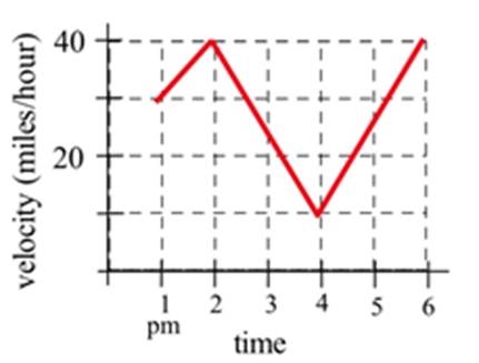
Write the total distance traveled by the car in the graph between 1 pm and 4 pm as a definite integral and estimate the value of the integral.
Problems 34 – 41 refer to the graph of \(f\) shown.
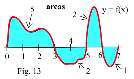
Use the graph to determine the values of the definite integrals. (The bold numbers represent the area of each region.)
| 34. \(\int^3_0 f(x) dx\) | 35. \(\int^5_3 f(x) dx\) | 36. \(\int^2_2 f(x) dx\) | 37. \(\int^7_6 f(w) dw\) |
| 38. \(\int^5_0 f(x) dx\) | 39. \(\int^7_0 f(x) dx\) | 40. \(\int^6_3 f(t) dt\) | 41. \(\int^7_5 f(x) dx\) |
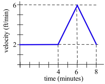
Problems 42 – 47 refer to the graph of \(g\) shown.
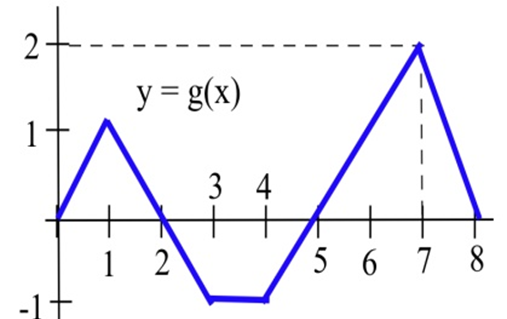
Use the graph to evaluate the integrals.
| 42. \(\int^2_0 g(x) dx\) | 43. \(\int^3_1 g(t) dt\) | 44. \(\int^5_0 g(x) dx\) |
| 45. \(\int^8_0 g(s) ds\) | 46. \(\int^3_0 2g(t) dt\) | 47. \(\int^8_5 1+g(x) dx\) |
3.2 Exercises
In problems 1 – 5, verify that \(F(x)\) is an antiderivative of the integrand \(f(x)\) and use Part 2 of the Fundamental Theorem to evaluate the definite integrals.
| 1. \(\int^1_0 2x dx, F(x) = x^2 + 5\) | 2. \(\int^4_1 3x^2 dx, F(x) = x^3 + 2\) | 3. \(\int^3_1 x^2 dx, F(x) = \frac{1}{3} x^3\) |
| 4. \(\int^3_0 (x^2+4x - 3) dx , F(x) = \frac{1}{3} x^3 + 2x^2 – 3x\) | 5. \(\int^5_1 \frac{1}{x} dx, F(x) = \ln ( x )\) |
Given \(A(x) = \int^x_0 2t dt\), find \(A'(x)\)
Given \(A(x) = \int^x_0 (3-t^2) dt\), find \(A'(x)\)
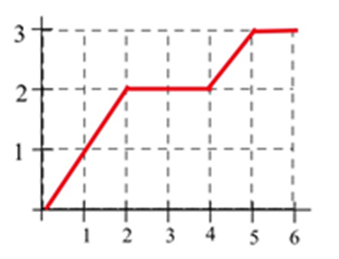
Let \(A(x) = \int^x_0 f(t) dt\) for the function graphed here.
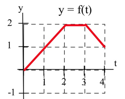
Evaluate \(A'(1)\), \(A'(2)\), \(A'(3)\).
For problems 9-10, the graph provided shows \(g'(x)\). Use it sketch a graph of \(g(x)\) that satisfies \(g(0) = 0\).
10.
3.3 Exercises
For problems 1-10, find the indicated antiderivative.
| 1. \(\int (x^3 - 14x + 5) dx\) | 2. \(\int (2.5x^5-x-1.25) dx\) |
| 3. \(\int 12.3 dy\) | 4. \(\int \pi^2 dw\) |
| 5. \(\int e^P dP\) | 6. \(\int \left( \sqrt{x} + e^x - \frac{1}{4x^3} \right) dx\) |
| 7. \(\int \frac{1}{x} dx\) | 8. \(\int \frac{1}{x^2} dx\) |
| 9. \(\int (x-2)(x+2) dx\) | 10. \(\int \frac{t^5-t^2}{t} dt\) |
For problems 11-18, find an antiderivative of the integrand and use the Fundamental Theorem to evaluate the definite integral.
| 11. \(\int^5_2 3x^2 dx\) | 12. \(\int^2_{-1} x^2 dx\) | 13. \(\int^3_1 (x^2+4x-3) dx\) | 14. \(\int^e_1 \frac{1}{x} dx\) |
| 15. \(\int^{100}_{25} \sqrt{x} dx\) | 16. \(\int^5_3 \sqrt{x} dx\) | 17. \(\int^{10}_1 \frac{1}{x^2} dx\) | 18. \(\int^{1000}_1 \frac{1}{x^2} dx\) |
For problems 19 - 21 find the area shown in the figure.
20.
3.4 Exercises
For problems 1-8, find the indicated antiderivative.
| 1. \(\int \frac{1}{(4x+1)^3} dx\) | 2. \(\int e^{100x} dx\) |
| 3. \(\int (1.0003)^{12t} dt\) | 4. \(\int \frac{e^{10/x}}{x^2} dx\) |
| 5. \(\int \sqrt{w+5} dw\) | 6. \(\int 6x^2 \sqrt{3x^3-1} dx\) |
| 7. \(\int \frac{dx}{x\ln x}\) | 8. \(\int \frac{x-3}{x^2-6x+5} dx\) |
For problems 9-12, find an antiderivative of the integrand and use the Fundamental Theorem to evaluate the definite integral.
| 9. \(\int^2_{-2} \frac{2x}{1+x^2} dx\) | 10. \(\int^1_0 e^{2x} dx\) | 11. \(\int^{4}_2 (x-2)^3 dx\) | 12. \(\int^1_0 x \sqrt{1-x^2} dx\) |
3.5 Exercises
In problems 1–4, a function \(u\) or \(dv\) is given. Find the piece \(u\) or \(dv\) which is not given, calculate \(du\) and \(v\), and apply the Integration by Parts Formula.
| 1. \(\int 12x \cdot \ln(x) dx\) | \(u = \ln(x)\) | 2. \(\int x \cdot e^{–x} dx\) | \(u = x\) |
| 3. \(\int x^4 \ln(x) dx\) | \(dv = x^4 dx\) | 4. \(\int x \cdot (5x + 1)^{19} dx\) | \(u = x\) |
In problems 5 - 10 evaluate the integrals
| 5. \(\int^1_0 \frac{x}{e^{3x}} dx\) | 6. \(\int^1_0 10x \cdot e^{3x} dx\) | 7. \(\int^3_1 \ln (2x + 5) dx\) |
| 8. \(\int x^3 \ln (5x) dx\) | 9. \(\int x \ln (x + 1) dx\) | 10. \(\int^2_1 \frac{\ln (x)}{x^2} dx\) |
For problems 11 - 14 integrate each function.
| 11. \(\int \frac{1}{4-x^2}\) | 12. \(\int \frac{2}{9-x^2}\) | 13. \(\int \sqrt{4+x^2}\) | 14. \(\int \sqrt{9+x^2}\) |
3.6 Exercises
In problems 1 – 4, use the values in the table to estimate the areas.
| \(x\) | \(f(x)\) | \(g(x)\) | \(h(x)\) |
|
0 |
5 |
2 |
5 |
|
1 |
6 |
1 |
6 |
|
2 |
6 |
2 |
8 |
|
3 |
4 |
2 |
6 |
|
4 |
3 |
3 |
5 |
|
5 |
2 |
4 |
4 |
|
6 |
2 |
0 |
2 |
1. Estimate the area between \(f\) and \(g\), between \(x = 0\) and \(x = 4\).
2. Estimate the area between \(g\) and \(h\), between \(x = 0\) and \(x = 6\).
3. Estimate the area between \(f\) and \(h\), between \(x = 0\) and \(x = 4\).
4. Estimate the area between \(f\) and \(g\), between \(x = 0\) and \(x = 6\).
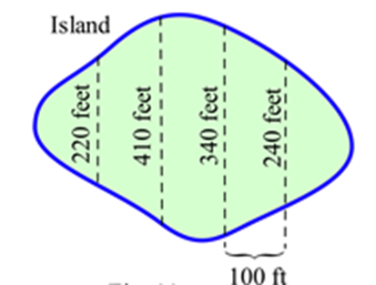
Estimate the area of the island shown
In problems 6 – 15, find the area between the graphs of \(f\) and \(g\) for \(x\) in the given interval. Remember to draw the graph!
| 6. \(f(x) = x^2 + 3 \), \(g(x) = 1\) and \(–1 \leq x \leq 2\). |
| 7. \(f(x) = x^2 + 3 \), \(g(x) = 1 + x\) and \(0 \leq x \leq 3\). |
| 8. \(f(x) = x^2 \), \(g(x) = x\) and \(0 \leq x \leq 2\). |
| 9. \(f(x) = (x –1)^2 \), \(g(x) = x + 1\) and \(0 \leq x \leq 3\). |
| 10. \(f(x) = \frac{1}{x}\), \(g(x) = x\) and \(1 \leq x \leq e\). |
| 11. \(f(x) = \sqrt{x}\), \(g(x) = x\) and \(0 \leq x \leq 4\). |
| 12. \(f(x) = 4 – x^2 \), \(g(x) = x + 2\) and \(0 \leq x \leq 2\). |
| 13. \(f(x) = e^x\), \(g(x) = x\) and \(0 \leq x \leq 2\). |
| 14. \(f(x) = 3 \), \(g(x) = \sqrt{1-x^2}\) and \(0 \leq x \leq 1\). |
| 15. \(f(x) = 2 \), \(g(x) = \sqrt{4-x^2}\) and \(–2 \leq x \leq 2\). |
For problems 16-18, find the volume of the solid obtained by rotating the specified region about the \(x\) axis.
16. Region under \(f(x) = x^2 + 3\) for \(–1 \leq x \leq 2\).
17. Region under \(f(x) = 4 – x^2\) for \(0 \leq x \leq 2\).
18. Region under \(f(x) = \frac{1}{x}\) for \(1 \leq x \leq 2\).
In problems 19 and 20 use the values in the table to estimate the average values.
| \(x\) | \(f(x)\) | \(g(x)\) |
|
0 |
5 |
2 |
|
1 |
6 |
1 |
|
2 |
6 |
2 |
|
3 |
4 |
2 |
|
4 |
3 |
3 |
|
5 |
2 |
4 |
|
6 |
2 |
0 |
19. Estimate the average value of \(f\) on the interval [0, 6].
20. Estimate the average value of \(g\) on the interval [0, 6].
In problems 21 – 26, find the average value of \(f\) on the given interval.
21. \(f(x)\) from the graph for \(0 \leq x \leq 2\).
22. \(f(x)\) from the graph for \(0 \leq x \leq 4\).
23. \(f(x)\) from the graph for \(1 \leq x \leq 6\).
24. \(f(x)\) from the graph for \(4 \leq x \leq 6\).
25. \(f(x) = 2x + 1\) for \(0 \leq x \leq 4\).
26. \(f(x) = x^2\) for \(0 \leq x \leq 2\).
The graph shows the velocity of a car during a 5 hour trip.
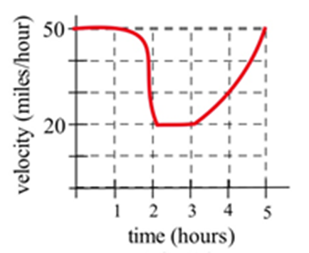
(a) Estimate how far the car traveled during the 5 hours.
(b) At what constant velocity should you drive in order to travel the same distance in 5 hours?
The graph shows the number of telephone calls per minute at a large company.
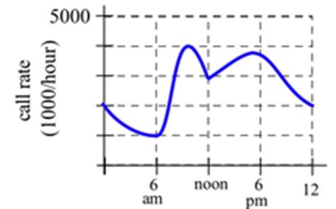
Estimate the average number of calls per minute
(a) From 8 am to 5 pm.
(b) From 9 am to 1 pm.
3.7 Exercises
The demand and supply functions for a certain product are given by \(p = 150 - .5q\) and \(p = .002q^2+1.5\), where \(p\) is in dollars and \(q\) is the number of items.
(a) Which is the demand function?
(b) Find the equilibrium price and quantity
(c) Find the total gains from trade at the equilibrium price.
Still thinking about the product from Exercise 1, with its demand and supply functions, suppose the price is set artificially at $70 (which is above the equilibrium price).
(a) Find the quantity supplied and the quantity demanded at this price.
(b) Compute the consumer surplus at this price, using the quantity demanded.
(c) Compute the producer surplus at this price, using the quantity demanded (why?).
(d) Find the total gains from trade at this price.
(e) What do you observe?
When the price of a certain product is $40, 25 items can be sold. When the price of the same product costs $20, 185 items can be sold. On the other hand, when the price of this product is $40, 200 items will be produced. But when the price of this product is $20, only 100 items will be produced. Use this information to find supply and demand functions (assume for simplicity that the functions are linear), and compute the consumer and producer surplus at the equilibrium price.
Find the present and future values of a continuous income stream of $5000 per year for 12 years if money can earn 1.3% annual interest compounded continuously.
Find the present value of a continuous income stream of $40,000 per year for 35 years if money can earn
(a) 0.8% annual interest, compounded continuously,
(b) 2.5% annual interest, compounded continuously,
(c) 4.5% annual interest, compounded continuously.
Find the present value of a continuous income stream \(F(t) = 20+t\), where \(t\) is in years and \(F\) is in tens of thousands of dollars per year, for 10 years, if money can earn 2% annual interest, compounded continuously.
Find the present value of a continuous income stream \(F(t) = 12+0.3t^t\), where \(t\) is in years and \(F\) is in thousands of dollars per year, for 8 years, if money can earn 3.7% annual interest, compounded continuously.
Find the future value of a continuous income stream \(F(t) = 8500+ \sqrt{640t+100}\), where \(t\) is in years and \(F\) is in dollars per year, for 15 years, if money can earn 6% annual interest, compounded continuously.
A business is expected to generate income at a continuous rate of $25,000 per year for the next eight years. Money can earn 3.4% annual interest, compounded continuously. The business is for sale for $153,000. Is this a good deal?
3.8 Exercises
In problems 1 – 4, check that the function \(y\) is a solution of the given differential equation.
| 1. \(y' + 3y = 6\). \(y = e^{–3x} + 2\). | 2. \(y' – 2y = 8\). \(y = e^{2x} – 4\). |
| 3. \(y' = – x/y\). \(y = \sqrt{7-x^2}\). | 4. \(y' = x – y\). \(y = x – 1 + 2e^{–x}\). |
In problems 5 – 8 check that the function \(y\) is a solution of the given initial value problem.
5. \(y' = 6x^2 – 3\) and \(y(1) = 2 \). \(y = 2x^3 – 3x + 3\).
6. \(y' = 6x + 4\) and \(y(2) = 3\). \(y = 3x^2 + 4x – 17\).
7. \(y' = 5y\) and \(y(0) = 7\). \(y = 7e^{5x}\).
8. \(y' = –2y\) and \(y(0) = 3\). \(y = 3e^{–2x}\).
In problems 9 – 12, a family of solutions of a differential equation is given. Find the value of the constant \(C\) so the solution satisfies the initial value condition.
| 9. \(y' = 2x\) and \(y(3) = 7\). \(y = x^2 + C\). | 10. \(y' = 3x^2 – 5\) and \(y(1) = 2\). \(y = x^3 – 5x + C\). |
| 11. \(y' = 3y\) and \(y(0) = 5\). \(y = Ce^{3x}\). | 12. \(y' = –2y\) and \(y(0) = 3\). \(y = Ce^{–2x}\). |
In problems 13 – 18, solve the differential equation. (Assume that \(x\) and \(y\) are restricted so that division by zero does not occur.)
| 13. \(y' = 2xy\) | 14. \(y' = x/y\) | 15. \(xy' = y + 3\) |
| 16. \(y' = x^2y + 3y\) | 17. \(y' = 4y\) | 18. \(y' = 5(2 – y)\) |
In problems 19 – 22, solve the initial value separable differential equations.
19. \(y' = 2xy\) for \(y(0) = 3\), \(y(0) = 5\), and \(y(1) = 2\).
20. \(y' = x/y\) for \(y(0) = 3\), \(y(0) = 5\), and \(y(1) = 2\).
21. \(y' = 3y\) for \(y(0) = 4\), \(y(0) = 7\), and \(y(1) = 3\).
22. \(y' = –2y\) for \(y(0) = 4\), \(y(0) = 7\), and \(y(1) = 3\).
The rate of growth of a population \(P(t)\) which starts with 3,000 people and increases by 4% per year is \(P '(t) = 0.0392 \cdot P(t)\). Solve the differential equation and use the solution to estimate the population in 20 years.
The rate of growth of a population \(P(t)\) which starts with 5,000 people and increases by 3% per year is \(P '(t) = 0.0296 \cdot P(t)\). Solve the differential equation and use the solution to estimate the population in 20 years.
A manufacturer estimates that she can sell a maximum of 130 thousand cell phones in a city. By advertising heavily, her total sales grow at a rate proportional to the distance below this upper limit. If she enters a new market, and after 6 months her total sales are 59 thousand phones, find a formula for the total sales (in thousands) \(t\) months after entering the market, and use this to estimate the total sales at the end of the first year.
The temperature of a turkey in the oven will grow like limited growth. The turkey starts out at 40 degrees Fahrenheit, and is placed into a 350 degree oven. After 30 minutes, the turkey's temperature has risen to 55 degrees. How long will it take until the turkey's temperature reaches 165 degrees?
A new cell phone is introduced into the market. It is predicted that sales will grow logistically. The manufacturer estimates that they can sell a maximum of 100 thousand cell phones. After 44 thousand cell phones have been sold, sales are increasing by 4 thousand phones per month. Use this to estimate the total sales at the end of the first year.
Biologists stocked a lake with 400 fish and estimated the carrying capacity of the lake to be 8000 fish. The number of fish tripled in the first year. How long will it take the population to increase to 4000?