
10.3E: Exercises for Section 10.3
- Page ID
- 72440

Taylor Polynomials
In exercises 1 - 8, find the Taylor polynomials of degree two approximating the given function centered at the given point.
1) \( f(x)=1+x+x^2\) at \( a=1\)
2) \( f(x)=1+x+x^2\) at \( a=−1\)
- Answer
- \( f(−1)=1;\;f′(−1)=−1;\;f''(−1)=2;\quad p_2(x)=1−(x+1)+(x+1)^2\)
3) \( f(x)=\cos(2x)\) at \( a=π\)
4) \( f(x)=\sin(2x)\) at \( a=\frac{π}{2}\)
- Answer
- \( f′(x)=2\cos(2x);\;f''(x)=−4\sin(2x);\quad p_2(x)=−2(x−\frac{π}{2})\)
5) \( f(x)=\sqrt{x}\) at \( a=4\)
6) \( f(x)=\ln x\) at \( a=1\)
- Answer
- \( f′(x)=\dfrac{1}{x};\; f''(x)=−\dfrac{1}{x^2};\quad p_2(x)=0+(x−1)−\frac{1}{2}(x−1)^2\)
7) \( f(x)=\dfrac{1}{x}\) at \( a=1\)
8) \( f(x)=e^x\) at \( a=1\)
- Answer
- \( p_2(x)=e+e(x−1)+\dfrac{e}{2}(x−1)^2\)
Taylor Remainder Theorem
In exercises 9 - 14, verify that the given choice of \(n\) in the remainder estimate \( |R_n|≤\dfrac{M}{(n+1)!}(x−a)^{n+1}\), where \(M\) is the maximum value of \( ∣f^{(n+1)}(z)∣\) on the interval between \(a\) and the indicated point, yields \( |R_n|≤\frac{1}{1000}\). Find the value of the Taylor polynomial \( p_n\) of \( f\) at the indicated point.
9) [T] \( \sqrt{10};\; a=9,\; n=3\)
10) [T] \( (28)^{1/3};\; a=27,\; n=1\)
- Answer
- \( \dfrac{d^2}{dx^2}x^{1/3}=−\dfrac{2}{9x^{5/3}}≥−0.00092…\) when \( x≥28\) so the remainder estimate applies to the linear approximation \( x^{1/3}≈p_1(27)=3+\dfrac{x−27}{27}\), which gives \( (28)^{1/3}≈3+\frac{1}{27}=3.\bar{037}\), while \( (28)^{1/3}≈3.03658.\)
11) [T] \( \sin(6);\; a=2π,\; n=5\)
12) [T] \( e^2; \; a=0,\; n=9\)
- Answer
- Using the estimate \( \dfrac{2^{10}}{10!}<0.000283\) we can use the Taylor expansion of order 9 to estimate \( e^x\) at \( x=2\). as \( e^2≈p_9(2)=1+2+\frac{2^2}{2}+\frac{2^3}{6}+⋯+\frac{2^9}{9!}=7.3887\)… whereas \( e^2≈7.3891.\)
13) [T] \( \cos(\frac{π}{5});\; a=0,\; n=4\)
14) [T] \( \ln(2);\; a=1,\; n=1000\)
- Answer
- Since \( \dfrac{d^n}{dx^n}(\ln x)=(−1)^{n−1}\dfrac{(n−1)!}{x^n},R_{1000}≈\frac{1}{1001}\). One has \(\displaystyle p_{1000}(1)=\sum_{n=1}^{1000}\dfrac{(−1)^{n−1}}{n}≈0.6936\) whereas \( \ln(2)≈0.6931⋯.\)
Approximating Definite Integrals Using Taylor Series
15) Integrate the approximation \(\sin t≈t−\dfrac{t^3}{6}+\dfrac{t^5}{120}−\dfrac{t^7}{5040}\) evaluated at \( π\)t to approximate \(\displaystyle ∫^1_0\frac{\sin πt}{πt}\,dt\).
16) Integrate the approximation \( e^x≈1+x+\dfrac{x^2}{2}+⋯+\dfrac{x^6}{720}\) evaluated at \( −x^2\) to approximate \(\displaystyle ∫^1_0e^{−x^2}\,dx.\)
- Answer
- \(\displaystyle ∫^1_0\left(1−x^2+\frac{x^4}{2}−\frac{x^6}{6}+\frac{x^8}{24}−\frac{x^{10}}{120}+\frac{x^{12}}{720}\right)\,dx =1−\frac{1^3}{3}+\frac{1^5}{10}−\frac{1^7}{42}+\frac{1^9}{9⋅24}−\frac{1^{11}}{120⋅11}+\frac{1^{13}}{720⋅13}≈0.74683\) whereas \(\displaystyle ∫^1_0e^{−x^2}dx≈0.74682.\)
More Taylor Remainder Theorem Problems
In exercises 17 - 20, find the smallest value of \(n\) such that the remainder estimate \( |R_n|≤\dfrac{M}{(n+1)!}(x−a)^{n+1}\), where \(M\) is the maximum value of \( ∣f^{(n+1)}(z)∣\) on the interval between \(a\) and the indicated point, yields \( |R_n|≤\frac{1}{1000}\) on the indicated interval.
17) \( f(x)=\sin x\) on \( [−π,π],\; a=0\)
18) \( f(x)=\cos x\) on \( [−\frac{π}{2},\frac{π}{2}],\; a=0\)
- Answer
- Since \( f^{(n+1)}(z)\) is \(\sin z\) or \(\cos z\), we have \( M=1\). Since \( |x−0|≤\frac{π}{2}\), we seek the smallest \(n\) such that \( \dfrac{π^{n+1}}{2^{n+1}(n+1)!}≤0.001\). The smallest such value is \( n=7\). The remainder estimate is \( R_7≤0.00092.\)
19) \( f(x)=e^{−2x}\) on \( [−1,1],a=0\)
20) \( f(x)=e^{−x}\) on \( [−3,3],a=0\)
- Answer
- Since \( f^{(n+1)}(z)=±e^{−z}\) one has \( M=e^3\). Since \( |x−0|≤3\), one seeks the smallest \(n\) such that \( \dfrac{3^{n+1}e^3}{(n+1)!}≤0.001\). The smallest such value is \( n=14\). The remainder estimate is \( R_{14}≤0.000220.\)
In exercises 21 - 24, the maximum of the right-hand side of the remainder estimate \( |R_1|≤\dfrac{max|f''(z)|}{2}R^2\) on \( [a−R,a+R]\) occurs at \(a\) or \( a±R\). Estimate the maximum value of \(R\) such that \( \dfrac{max|f''(z)|}{2}R^2≤0.1\) on \( [a−R,a+R]\) by plotting this maximum as a function of \(R\).
21) [T] \( e^x\) approximated by \( 1+x,\; a=0\)
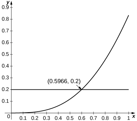
22) [T] \( \sin x\) approximated by \( x,\; a=0\)
- Answer
-
Since \( \sin x\) is increasing for small \( x\) and since \( \frac{d^2}{dx^2}\left(\sin x\right)=−\sin x\), the estimate applies whenever \( R^2\sin(R)≤0.2\), which applies up to \( R=0.596.\)
23) [T] \( \ln x\) approximated by \( x−1,\; a=1\)
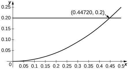
24) [T] \( \cos x\) approximated by \( 1,\; a=0\)
- Answer
-
Since the second derivative of \( \cos x\) is \( −\cos x\) and since \( \cos x\) is decreasing away from \( x=0\), the estimate applies when \( R^2\cos R≤0.2\) or \( R≤0.447\).
Taylor Series
In exercises 25 - 35, find the Taylor series of the given function centered at the indicated point.
25) \(f(x) = x^4\) at \( a=−1\)
26) \(f(x) = 1+x+x^2+x^3\) at \( a=−1\)
- Answer
- \( (x+1)^3−2(x+1)^2+2(x+1)\)
27) \(f(x) = \sin x\) at \( a=π\)
28) \(f(x) = \cos x\) at \( a=2π\)
- Answer
- Values of derivatives are the same as for \( x=0\) so \(\displaystyle \cos x=\sum_{n=0}^∞(−1)^n\frac{(x−2π)^{2n}}{(2n)!}\)
29) \(f(x) = \sin x\) at \( x=\frac{π}{2}\)
30) \(f(x) = \cos x\) at \( x=\frac{π}{2}\)
- Answer
- \( \cos(\frac{π}{2})=0,\;−\sin(\frac{π}{2})=−1\) so \(\displaystyle \cos x=\sum_{n=0}^∞(−1)^{n+1}\frac{(x−\frac{π}{2})^{2n+1}}{(2n+1)!}\), which is also \( −\cos(x−\frac{π}{2})\).
31) \(f(x) = e^x\) at \( a=−1\)
32) \(f(x) = e^x\) at \( a=1\)
- Answer
- The derivatives are \( f^{(n)}(1)=e,\) so \(\displaystyle e^x=e\sum_{n=0}^∞\frac{(x−1)^n}{n!}.\)
33) \(f(x) = \dfrac{1}{(x−1)^2}\) at \( a=0\) (Hint: Differentiate the Taylor Series for\( \dfrac{1}{1−x}\).)
34) \(f(x) = \dfrac{1}{(x−1)^3}\) at \( a=0\)
- Answer
- \(\displaystyle \frac{1}{(x−1)^3}=−\frac{1}{2}\frac{d^2}{dx^2}\left(\frac{1}{1−x}\right)=−\sum_{n=0}^∞\left(\frac{(n+2)(n+1)x^n}{2}\right)\)
35) \(\displaystyle F(x)=∫^x_0\cos(\sqrt{t})\,dt;\quad \text{where}\; f(t)=\sum_{n=0}^∞(−1)^n\frac{t^n}{(2n)!}\) at a=0 (Note: \( f\) is the Taylor series of \(\cos(\sqrt{t}).)\)
In exercises 36 - 44, compute the Taylor series of each function around \( x=1\).
36) \( f(x)=2−x\)
- Answer
- \( 2−x=1−(x−1)\)
37) \( f(x)=x^3\)
38) \( f(x)=(x−2)^2\)
- Answer
- \( ((x−1)−1)^2=(x−1)^2−2(x−1)+1\)
39) \( f(x)=\ln x\)
40) \( f(x)=\dfrac{1}{x}\)
- Answer
- \(\displaystyle \frac{1}{1−(1−x)}=\sum_{n=0}^∞(−1)^n(x−1)^n\)
41) \( f(x)=\dfrac{1}{2x−x^2}\)
42) \( f(x)=\dfrac{x}{4x−2x^2−1}\)
- Answer
- \(\displaystyle x\sum_{n=0}^∞2^n(1−x)^{2n}=\sum_{n=0}^∞2^n(x−1)^{2n+1}+\sum_{n=0}^∞2^n(x−1)^{2n}\)
43) \( f(x)=e^{−x}\)
44) \( f(x)=e^{2x}\)
- Answer
- \(\displaystyle e^{2x}=e^{2(x−1)+2}=e^2\sum_{n=0}^∞\frac{2^n(x−1)^n}{n!}\)
Maclaurin Series
[T] In exercises 45 - 48, identify the value of \(x\) such that the given series \(\displaystyle \sum_{n=0}^∞a_n\) is the value of the Maclaurin series of \( f(x)\) at \( x\). Approximate the value of \( f(x)\) using \(\displaystyle S_{10}=\sum_{n=0}^{10}a_n\).
45) \(\displaystyle \sum_{n=0}^∞\frac{1}{n!}\)
46) \(\displaystyle \sum_{n=0}^∞\frac{2^n}{n!}\)
- Answer
- \( x=e^2;\quad S_{10}=\dfrac{34,913}{4725}≈7.3889947\)
47) \(\displaystyle \sum_{n=0}^∞\frac{(−1)^n(2π)^{2n}}{(2n)!}\)
48) \(\displaystyle \sum_{n=0}^∞\frac{(−1)^n(2π)^{2n+1}}{(2n+1)!}\)
- Answer
- \(\sin(2π)=0;\quad S_{10}=8.27×10^{−5}\)
In exercises 49 - 52 use the functions \( S_5(x)=x−\dfrac{x^3}{6}+\dfrac{x^5}{120}\) and \( C_4(x)=1−\dfrac{x^2}{2}+\dfrac{x^4}{24}\) on \( [−π,π]\).
49) [T] Plot \(\sin^2x−(S_5(x))^2\) on \( [−π,π]\). Compare the maximum difference with the square of the Taylor remainder estimate for \( \sin x.\)
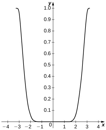
50) [T] Plot \(\cos^2x−(C_4(x))^2\) on \( [−π,π]\). Compare the maximum difference with the square of the Taylor remainder estimate for \( \cos x\).
- Answer
-
The difference is small on the interior of the interval but approaches \( 1\) near the endpoints. The remainder estimate is \( |R_4|=\frac{π^5}{120}≈2.552.\)
51) [T] Plot \( |2S_5(x)C_4(x)−\sin(2x)|\) on \( [−π,π]\).
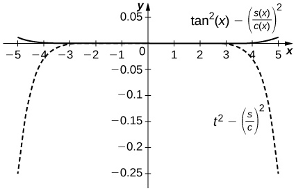
52) [T] Compare \( \dfrac{S_5(x)}{C_4(x)}\) on \( [−1,1]\) to \( \tan x\). Compare this with the Taylor remainder estimate for the approximation of \( \tan x\) by \( x+\dfrac{x^3}{3}+\dfrac{2x^5}{15}\).
- Answer
-
The difference is on the order of \( 10^{−4}\) on \( [−1,1]\) while the Taylor approximation error is around \( 0.1\) near \( ±1\). The top curve is a plot of \(\tan^2x−\left(\dfrac{S_5(x)}{C_4(x)}\right)^2\) and the lower dashed plot shows \( t^2−\left(\dfrac{S_5}{C_4}\right)^2\).
53) [T] Plot \( e^x−e_4(x)\) where \( e_4(x)=1+x+\dfrac{x^2}{2}+\dfrac{x^3}{6}+\dfrac{x^4}{24}\) on \( [0,2]\). Compare the maximum error with the Taylor remainder estimate.
54) (Taylor approximations and root finding.) Recall that Newton’s method \( x_{n+1}=x_n−\dfrac{f(x_n)}{f'(x_n)}\) approximates solutions of \( f(x)=0\) near the input \( x_0\).
a. If \( f\) and \( g\) are inverse functions, explain why a solution of \( g(x)=a\) is the value \( f(a)\) of \( f\).
b. Let \( p_N(x)\) be the \( N^{\text{th}}\) degree Maclaurin polynomial of \( e^x\). Use Newton’s method to approximate solutions of \( p_N(x)−2=0\) for \( N=4,5,6.\)
c. Explain why the approximate roots of \( p_N(x)−2=0\) are approximate values of \(\ln(2).\)
- Answer
- a. Answers will vary.
b. The following are the \( x_n\) values after \( 10\) iterations of Newton’s method to approximation a root of \( p_N(x)−2=0\): for \( N=4,x=0.6939...;\) for \( N=5,x=0.6932...;\) for \( N=6,x=0.69315...;.\) (Note: \( \ln(2)=0.69314...\))
c. Answers will vary.
Evaluating Limits using Taylor Series
In exercises 55 - 58, use the fact that if \(\displaystyle q(x)=\sum_{n=1}^∞a_n(x−c)^n\) converges in an interval containing \( c\), then \(\displaystyle \lim_{x→c}q(x)=a_0\) to evaluate each limit using Taylor series.
55) \(\displaystyle \lim_{x→0}\frac{\cos x−1}{x^2}\)
56) \(\displaystyle \lim_{x→0}\frac{\ln(1−x^2)}{x^2}\)
- Answer
- \( \dfrac{\ln(1−x^2)}{x^2}→−1\)
57) \(\displaystyle \lim_{x→0}\frac{e^{x^2}−x^2−1}{x^4}\)
58) \(\displaystyle \lim_{x→0^+}\frac{\cos(\sqrt{x})−1}{2x}\)
- Answer
- \(\displaystyle \frac{\cos(\sqrt{x})−1}{2x}≈\frac{(1−\frac{x}{2}+\frac{x^2}{4!}−⋯)−1}{2x}→−\frac{1}{4}\)