8.4: Alternating Series

Learning Objectives

In this section, we strive to understand the ideas generated by the following important questions:

• What is an alternating series?
• What does it mean for an alternating series to converge?
• Under what conditions does an alternating series converge? Why?
• How well does the nth partial sum of a convergent alternating series approximate the actual sum of the series? Why?
• What is the difference between absolute convergence and conditional convergence?

In our study of series so far, almost every series that we’ve considered has exclusively nonnegative terms. Of course, it is possible to consider series that have some negative terms. For instance, if we consider the geometric series

\[2 − \dfrac{4}{3} + \dfrac{8}{9} − \ldots + 2 \left(\dfrac{−2}{3}\right)^n + \ldots , \]

which has \(a = 2\) and \(r = − \dfrac{2}{3}\), we see that not only does every other term alternate in sign, but also that this series converges to

\[S = \dfrac{a}{1 − r} = \dfrac{2}{1 − \left(− \dfrac{2}{3}\right) } = \dfrac{6}{5}. \]

In Preview Activity \(\PageIndex{1}\) and our following discussion, we investigate the behavior of similar series where consecutive terms have opposite signs.

Preview Activity \(\PageIndex{1}\)

showed how we can approximate the number e with linear, quadratic, and other polynomial approximations. We use a similar approach in this activity to obtain linear and quadratic approximations to \( \ln(2)\). Along the way, we encounter a type of series that is different than most of the ones we have seen so far. Throughout this activity, let \(f (x) = \ln(1 + x)\).

a. Find the tangent line to \(f\) at \(x = 0\) and use this linearization to approximate \( \ln(2)\). That is, find \(L(x)\), the tangent line approximation to \(f (x)\), and use the fact that \(L(1) \approx f (1)\) to estimate \(\ln(2)\).

b. The linearization of \( \ln(1 + x)\) does not provide a very good approximation to \( \ln(2)\) since 1 is not that close to 0. To obtain a better approximation, we alter our approach; instead of using a straight line to approximate \( \ln(2)\), we use a quadratic function to account for the concavity of \( \ln(1 + x)\) for \(x\) close to 0. With the linearization, both the function’s value and slope agree with the linearization’s value and slope at \(x = 0\). We will now make a quadratic approximation \(P_2(x) to f (x)\) = \(\ln(1 + x) \) centered at \(x = 0\) with the property that \(P_2(0) = f (0), P'_2 (0) = f'(0)\), and \(P''_2 (0) = f''(0)\).

1. Let \(P_2(x) = x − \dfrac{x^2}{2}\). Show that \(P_2(0) = f (0), P'_2 (0) = f'(0)\), and \(P''2 (0) = f''(0)\). Use \(P_2(x)\) to approximate \(\ln(2)\) by using the fact that \(P_2(1) \approx f (1)\).
2. We can continue approximating \( \ln(2)\) with polynomials of larger degree whose derivatives agree with those of \(f\) at 0. This makes the polynomials fit the graph of \(f\) better for more values of \(x\) around 0. For example, let \(P_3(x) = x − \dfrac{x^2}{2} + \dfrac{x^3}{3}\). Show that \(P_3(0) = f (0), P'_3 (0) = f'(0), P''_3 (0) = f''(0)\), and \(P'''_3 (0) = f'''(0)\). Taking a similar approach to preceding questions, use P3(x) to approximate \( \ln(2)\).
3. If we used a degree 4 or degree 5 polynomial to approximate \( \ln(1 + x)\), what approximations of \( \ln(2)\) do you think would result? Use the preceding questions to conjecture a pattern that holds, and state the degree 4 and degree 5 approximation. .

Preview Activity \(\PageIndex{1}\) gives us several approximations to \(\ln(2)\), the linear approximation is 1 and the quadratic approximation is \(1 − \dfrac{1}{2} = \dfrac{1}{2} \). If we continue this process we will obtain approximations from cubic, quartic (degree 4), quintic (degree 5), and higher degree polynomials giving us the following approximations to \(ln(2)\):

Linear	1	1
Quadratric	\(1- \dfrac{1}{2}\)	0.5
Cubic	\(1- \dfrac{1}{2}+ \dfrac{1}{3}\)	0.83̅
Quartic	\(1- \dfrac{1}{2}+ \dfrac{1}{3} - \dfrac{1}{4}\)	0.583̅
Quintic	\(1- \dfrac{1}{2}+ \dfrac{1}{3} - \dfrac{1}{4}+ \dfrac{1}{5}\)	0.783̅

The pattern here shows the fact that the number \(ln(2)\) can be approximated by the partial sums of the infinite series

\[\sum_{k=1}^\infty (-1)^{k+1} \frac{1}{k} \tag{8.15} \label{8.15}\]

where the alternating signs are determined by the factor \((−1)^{k+1}\). Using computational technology, we find that 0.6881721793 is the sum of the first 100 terms in this series. As a comparison, \(\ln(2) \approx\) 0.6931471806. This shows that even though the series (Equation \(\ref{8.15}\)) converges to \( \ln(2)\), it must do so quite slowly, since the sum of the first 100 terms isn’t particularly close to \( \ln(2)\). We will investigate the issue of how quickly an alternating series converges later in this section. Again, note particularly that the series \(\ref{8.15}\) is different from the series we have considered earlier in that some of the terms are negative. We call such a series an alternating series.

Definition: alternating series

An alternating series is a series of the form

\[\sum_{k=0}^{\infty} (−1)^k a_k, \nonumber\]

where \(a_k ≥ 0\) for each \(k\). We have some flexibility in how we write an alternating series; for example, the series

\[\sum_{k=1}^{\infty} (−1)^{k+1} a_k, \nonumber\]

whose index starts at \(k = 1\), is also alternating. As we will soon see, there are several very nice results that hold about alternating series, while alternating series can also demonstrate some unusual behavior.

It is important to remember that most of the series tests we have seen in previous sections apply only to series with nonnegative terms. Thus, alternating series require a different test. To investigate this idea, we return to the example in Preview Activity \(\PageIndex{1}\).

Activity \(\PageIndex{1}\)

Remember that, by definition, a series converges if and only if its corresponding sequence of partial sums converges.

Complete Table 8.7 by calculating the first few partial sums (to 10 decimal places) of the alternating series

\[\sum_{k=1}^{\infty} (−1)^{k+1} \dfrac{1}{k}. \nonumber\]

Plot the sequence of partial sums from part (a) in the plane. What do you notice about this sequence?

Activity \(\PageIndex{1}\) exemplifies the general behavior that any convergent alternating series will demonstrate. In this example, we see that the partial sums of the alternating harmonic series oscillate around a fixed number that turns out to be the sum of the series.

Table 8.7: Partial sums of the alternating series \(\sum_{k=1}^{\infty} (−1)^{k+1} \dfrac{1}{k}\)

\(\sum_{k=1}^{1} (−1)^{k+1} \dfrac{1}{k}\)=	\(\sum_{k=1}^{6} (−1)^{k+1} \dfrac{1}{k}\)=
\(\sum_{k=1}^{2} (−1)^{k+1} \dfrac{1}{k}\)=	\(\sum_{k=1}^{7} (−1)^{k+1} \dfrac{1}{k}\)=
\(\sum_{k=1}^{3} (−1)^{k+1} \dfrac{1}{k}\)=	\(\sum_{k=1}^{8} (−1)^{k+1} \dfrac{1}{k}\)=
\(\sum_{k=1}^{4} (−1)^{k+1} \dfrac{1}{k}\)=	\(\sum_{k=1}^{9} (−1)^{k+1} \dfrac{1}{k}\)=
\(\sum_{k=1}^{5} (−1)^{k+1} \dfrac{1}{k}\)=	\(\sum_{k=1}^{10} (−1)^{k+1} \dfrac{1}{k}\)

Recall that if \(\lim_{k→∞} a^k \neq 0\), then the series \(P a^k\) diverges by the Divergence Test. From this point forward, we will thus only consider alternating series

\[\sum_{k=1}^{\infty} (−1)^{k+1} a_k \nonumber\]

in which the sequence \(a_k\) consists of positive numbers that decrease to 0. For such a series, the \(n\)th partial sum \(S_n\) satisfies

\[S_n = \sum_{k=1}^n (-1)^{k+1} a_k. \nonumber\]

Notice that

• \(S_1 = a_1\)
• \(S_2 = a_1 − a_2\), and since \(a_1 > a_2\) we have

\[0 < S_2 < S_1. \nonumber\]

• \(S_3 = S_2 + a_3\) and so \(S_2 < S_3\). But \(a_3 < a_2\), so \(S_3 < S_1\). Thus,

\[0 < S_2 < S_3 < S_1 \nonumber\]

• \(S_4 = S_3 − a_4\) and so \(S_4 < S_3\). But \(a_4 < a_3\), so \(S_2 < S_4\). Thus,

\[0 < S_2 < S_4 < S_3 < S_1. \nonumber\]

• \(S_5 = S_4 + a_5\) and so \(S_4 < S_5\). But \(a_5 < a_4\), so \(S_5 < S_3\). Thus,

\[0 < S_2 < S_4 < S_5 < S_3 < S_1. \nonumber\]

This pattern continues as illustrated in Figure \(\PageIndex{1}\) (with \(n\) odd) so that each partial sum lies between the previous two partial sums. Note further that the absolute value of the difference between the \((n − 1)\)st partial sum \(S_n−1\) and the nth partial sum \(S_n\) is

\[|S_n − S_n−1| = a_n. \nonumber\]

Since the sequence {\(a_n\)} converges to 0, the distance between successive partial sums becomes as close to zero as we’d like, and thus the sequence of partial sums converges (even though we don’t know the exact value to which the sequence of partial sums converges). The preceding discussion has demonstrated the truth of the Alternating Series Test.

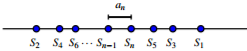
Figure \(\PageIndex{1}\): Partial sums of an alternating series

Definition: The Alternating Series Test

Given an alternating series

\[\sum (−1)^k a_k, \nonumber\]

if the sequence \(\{a_k \}\) of positive terms decreases to 0 as \(k \rightarrow \infty\), then the alternating series converges.

Note particularly that if the limit of the sequence {\(a_k\) } is not 0, then the alternating series diverges.

Activity \(\PageIndex{2}\)

Which series converge and which diverge? Justify your answers.

1. \(\sum_{k=1}^{\infty} \dfrac{(−1)^k}{k^2 + 2}\)
2. \(\sum_{k=1}^{\infty} \dfrac{(−1)^{k+1} 2k}{k + 5} \)
3. \(\sum_{k=2}^{\infty} \dfrac{(−1)^k}{\ln(k)}\)

The argument for the Alternating Series Test also provides us with a method to determine how close the \(n\)th partial sum \(S_n\) is to the actual sum of a convergent alternating series. To see how this works, let \(S\) be the sum of a convergent alternating series, so

\[S = \sum_{k=1}^{\infty} (−1)^k a_k . \nonumber\]

Recall that the sequence of partial sums oscillates around the sum \(S\) so that

\[|S − S_n| < |S_{n+1} − S_n| = a_{n+1}. \nonumber\]

Therefore, the value of the term an+1 provides an error estimate for how well the partial sum \(S_n\) approximates the actual sum \(S\). We summarize this fact in the statement of the Alternating Series Estimation Theorem.

Alternating Series Estimation Theorem

If the alternating series

\[\sum_{k=1}^{\infty} (−1)^{k+1} a_k \nonumber\]

converges and has sum \(S\), and

\[S_n = \sum^n_{ k=1} (−1)^{ k+1} a_k \nonumber\]

is the nth partial sum of the alternating series, then

\[ | \sum_{k=1}^{\infty} (−1)^{k+1} a_k − S_n | ≤ a_n+1. \nonumber\]

Example \(\PageIndex{1}\)

Let’s determine how well the 100th partial sum \(S_{100}\) of

\[\sum_{k=1}^{\infty} \dfrac{(−1)^{k+1}}{k} \nonumber\]

approximates the sum of the series.

Solution.

If we let S be the sum of the series P∞ k=1 (−1) k+1 k , then we know that

\[ |S100 − S| < a_{101}. \nonumber\]

Now

\[a_{101} = \dfrac{1}{101} \approx 0.0099, \nonumber\]

so the 100th partial sum is within 0.0099 of the sum of the series. We have discussed the fact (and will later verify) that

\[S = \sum_{k=1}^{\infty} \dfrac{(−1)^{k+1}}{k} = ln(2) , \nonumber\]

and so \( S \approx 0.693147\) while

\[S_{100} =\sum_{k=1}^{\infty} \dfrac{(−1)^{k+1}}{k} \approx 0.6881721793. \nonumber\]

We see that the actual difference between S and \(S_{100}\) is approximately 0.0049750013, which is indeed less than 0.0099.

Activity \(\PageIndex{3}\)

Determine the number of terms it takes to approximate the sum of the convergent alternating series

\[\sum_{k=1}^{\infty} \dfrac{(−1)^{ k+1}}{ k^ 4} \nonumber\]

to within 0.0001.

Absolute and Conditional Convergence

A series such as

\[1 − \dfrac{1}{4} − \dfrac{1}{9} + \dfrac{1}{16} + \dfrac{1}{25} + \dfrac{1}{36} − \dfrac{1}{49} − \dfrac{1}{64} − \dfrac{1}{81} − \dfrac{1}{100} + \ldots \tag{8.16}\label{8.16}\]

whose terms are neither all nonnegative nor alternating is different from any series that we have considered to date. The behavior of these series can be rather complicated, but there is an important connection between these arbitrary series that have some negative terms and series with all nonnegative terms that we illustrate with the next activity.

Activity \(\PageIndex{4}\)

a. Explain why the series

\[1 − \dfrac{1}{4} − \dfrac{1}{9} + \dfrac{1}{16} + \dfrac{1}{ 25} + \dfrac{1} {36} − \dfrac{1}{49} − \dfrac{1}{64} − \dfrac{1}{81} − \dfrac{1}{100} + \ldots\]

must have a sum that is less than the series

\[\sum_{k=1}^{\infty} \dfrac{1}{ k^2}. \nonumber\]

b. Explain why the series

\[1 − \dfrac{1}{4} − \dfrac{1}{9} + \dfrac{1}{16} + \dfrac{1}{ 25} + \dfrac{1} {36} − \dfrac{1}{49} − \dfrac{1}{64} − \dfrac{1}{81} − \dfrac{1}{100} + \ldots \nonumber\]

must have a sum that is greater than the series

\[\sum_{k=1}^{\infty} - \dfrac{1}{ k^2}. \nonumber\]

c. Given that the terms in the series

\[1 − \dfrac{1}{4} − \dfrac{1}{9} + \dfrac{1}{16} + \dfrac{1}{ 25} + \dfrac{1} {36} − \dfrac{1}{49} − \dfrac{1}{64} − \dfrac{1}{81} − \dfrac{1}{100} + \ldots \nonumber\]

converge to 0, what do you think the previous two results tell us about the convergence status of this series?

As the example in Activity \(\PageIndex{4}\)suggests, if we have a series \(\sum a_k\), (some of whose terms may be negative) such that \(\sum |a_k | \) converges, it turns out to always be the case that the original series, \(\sum a_k\), must also converge. That is, if \(\sum |a_k | \) converges, then so must \(\sum a_k\).

As we just observed, this is the case for the series (8.16), since the corresponding series of the absolute values of its terms is the convergent p-series \(\sum d\frac{1}{k^2}\). At the same time, there are series like the alternating harmonic series \(\sum (−1)^{k+1} \dfrac{1}{k}\) that converge, while the corresponding series of absolute values, \( \sum \dfrac{1}{k}\), diverges. We distinguish between these behaviors by introducing the following language.

Definition

Consider a series \(\sum a_k\)

1. The series \(\sum a_k\) converges absolutely (or is absolutely convergent) provided that \(\sum |a_k | \) converges.
2. The series \(\sum a_k\) converges conditionally (or is conditionally convergent) provided that \(\sum |a_k | \) diverges and \(\sum a_k\) converges

In this terminology, the series (Equation \ref{8.16}) converges absolutely while the alternating harmonic series is conditionally convergent.

Activity \(\PageIndex{5}\):

a. Consider the series \(\sum (-1)^k \dfrac{\ln(k)}{k}\).

1. Does this series converge? Explain.
2. Does this series converge absolutely? Explain what test you use to determine your answer.

b. Consider the series \(\sum (-1)^k \dfrac{\ln(k)}{k^2}\).

1. Does this series converge? Explain.
2. Does this series converge absolutely? Hint: Use the fact that \( \ln(k) < \sqrt{k}\) for large values of \(k\) and the compare to an appropriate \(p\)-series.

Conditionally convergent series turn out to be very interesting. If the sequence {\(a_n\)} decreases to 0, but the series \(\sum a_k\) diverges, the conditionally convergent series \(\sum (−1)^k a_k\) is right on the borderline of being a divergent series. As a result, any conditionally convergent series converges very slowly. Furthermore, some very strange things can happen with conditionally convergent series, as illustrated in some of the exercises.

Summary of Tests for Convergence of Series

We have discussed several tests for convergence/divergence of series in our sections and in exercises. We close this section of the text with a summary of all the tests we have encountered, followed by an activity that challenges you to decide which convergence test to apply to several different series.

Geometric Series

The geometric series \(\sum ar^k\) with ratio \(r\) converges for \(−1 < r < 1 \) and diverges for \(|r| ≥ 1\).

The sum of the convergent geometric series \(\sum_{k=0}^\infty ar^k \) is \(\dfrac{a}{1-r}\)

Divergence Test

If the sequence \(a_n\) does not converge to 0, then the series \(\sum a_k\) diverges.

This is the first test to apply because the conclusion is simple. However, if \(\lim_{n \rightarrow \infty} a_n = 0 \), no conclusion can be drawn

Integral Test

Let \(f\) be a positive, decreasing function on an interval \([c, \infty]\) and let \(a_k = f (k)\) for each positive integer \(k ≥ c\).

• If \( \int_{c}^{\infty} f(t) dt\) converges, then \(\sum a_k\) converges.
• If \( \int_{c}^{\infty} f(t) dt\) diverges, then \(\sum a_k\) diverges.

Use this test when \(f (x)\) is easy to integrate.

Direct Comparison Test

See Ex 4 in Section 8.3 .

Let \(0 ≤ a_k ≤ b_k\) for each positive integer \(k\).

• If \(\sum b_k\) converges, then \(\sum a_k\) converges.
• If \(\sum a_k\) diverges, then \(\sum b_k\) diverges

Use this test when you have a series with known behavior that you can compare to – this test can be difficult to apply.

Limit Comparison Test

Let an and bn be sequences of positive terms. If

\[ \lim_{k \rightarrow \infty} \dfrac{a_k}{b_k} = L \nonumber\]

for some positive finite number \(L\), then the two series \(\sum a_k\) and \(\sum b_k\) either both converge or both diverge.

Easier to apply in general than the comparison test, but you must have a series with known behavior to compare. Useful to apply to series of rational functions.

Ratio test

Let \( a_k \neq 0\) for each \(k\) and suppose

\[ \lim_{k \rightarrow \infty} \dfrac{ |ak+1|}{ |ak |} = r. \nonumber\]

• If \(r < 1\), then the series \(\sum a_k\) converges absolutely.
• If \(r > 1\), then the series \(\sum a_k\) diverges.
• If \(r = 1\), then test is inconclusive.

This test is useful when a series involves factorials and powers.

Root Test

Let \(a_k ≥ 0\) for each \(k\) and suppose

\[ \lim_{k \rightarrow \infty} \sqrt[k]{a_k}=r. \nonumber\]

• If \(r < 1\), then the series \(\sum a_k\) converges.
• If \(r > 1\), then the series \(\sum a_k\) diverges.
• If \(r = 1\), then test is inconclusive.

In general, the Ratio Test can usually be used in place of the Root Test. However, the Root Test can be quick to use when \(a_k\) involves \(k\)th powers.

Alternating Series Test

If \(a_n\) is a positive, decreasing sequence so that \(\lim_{k \rightarrow \infty} a_n = 0\), then the alternating series \( \sum (−1)^{k+1} a_k\) converges.

This test applies only to alternating series – we assume that the terms \(a_n\) are all positive and that the sequence {\(a_n\)} is decreasing.

Alternating Series Estimation Theorem

Let \(S_n = \sum_{k=1}^n(-1)^{k+1}a_k\) be the \(n\)th partial sum of the alternating series \( \sum_{k=1}^n(-1)^{k+1}a_k\). Assume \(a_n > 0\) for each positive integer \(n\), the sequence an decreases to 0 and \(\lim_{n \rightarrow \infty} S_n = S\). Then it follows that \(|S − S_n| < a_n+1\.

This bound can be used to determine the accuracy of the partial sum \(S_n\) as an approximation of the sum of a convergent alternating series.

Activity \(\PageIndex{6}\):

For (a)-(j), use appropriate tests to determine the convergence or divergence of the following series. Throughout, if a series is a convergent geometric series, find its sum.

1. \(\sum_{k=3}^{\infty} \dfrac{2}{\sqrt{ k − 2}}\)
2. \(\sum_{k=1}^{\infty} \dfrac{k}{1 + 2k}\)
3. \(\sum_{k=0}^{\infty} \dfrac{2k^2 + 1}{k^3 + k + 1}\)
4. \(\sum_{k=0}^{\infty} \dfrac{100^k}{k!}\)
5. \(\sum_{k=1}^{\infty}\dfrac{2^k}{5^k}\)
6. \( \sum_{k=1}^{\infty} \dfrac{k^3 − 1}{k^5 + 1}\)
7. \(\sum_{k=2}^{\infty} \dfrac{3^{k−1}{7^k}\)
8. \( \sum_{k=2}^{\infty} \dfrac{1}{k^k}\)
9. \(\sum_{k=1}^{\infty} \dfrac{ (−1)^{k+1}}{\sqrt{k+1}}\)
10. \(\sum_{k=2}^{\infty} \dfrac{1}{k \ln(k)}\)
11. Determine a value of \(n\) so that the nth partial sum \(S_n\) of the alternating series \(\sum_{n=2}^\infty \dfrac{(-1)^n}{\ln(n)}\) approximates the sum to within 0.001.

Summary

In this section, we encountered the following important ideas:

• An alternating series is a series whose terms alternate in sign. In other words, an alternating series is a series of the form

\[ \sum (−1)^k a_k \nonumber\]

where \(a_k\) is a positive real number for each \(k\).

• An alternating series \(\sum_{k=1}^\infty (−1)^k a_k\). converges if and only if its sequence {\(S_n\)} of partial sums converges, where

\[S_n = \sum_{k=1}^n (−1)^k a_k. \nonumber\]

• The sequence of partial sums of a convergent alternating series oscillates around and converge to the sum of the series if the sequence of \(n\)th terms converges to 0. That is why the Alternating Series Test shows that the alternating series \(\sum_{k=1}^\infty (−1)^k a_k\) converges whenever the sequence {\(a_n\)} of nth terms decreases to 0.
• The difference between the \(n\) − 1st partial sum \(S_{n−1}\) and the \(n\)th partial sum \(S_n\) of a convergent alternating series \(\sum_{k=1}^\infty (−1)^k a_k\) is \(|S_n − S_{n-1}| = a_n\).. Since the partial sums oscillate around the sum S of the series, it follows that

\[|S − S_n| < a_n. \nonumber\]

• So the \(n\)th partial sum of a convergent alternating series \(\sum_{k=1}^\infty (−1)^k a_k\) approximates the actual sum of the series to within \(a_n\).