
14.7: Maxima/Minima Problems
- Page ID
- 2606

- Use partial derivatives to locate critical points for a function of two variables.
- Apply a second derivative test to identify a critical point as a local maximum, local minimum, or saddle point for a function of two variables.
- Examine critical points and boundary points to find absolute maximum and minimum values for a function of two variables.
One of the most useful applications for derivatives of a function of one variable is the determination of maximum and/or minimum values. This application is also important for functions of two or more variables, but as we have seen in earlier sections of this chapter, the introduction of more independent variables leads to more possible outcomes for the calculations. The main ideas of finding critical points and using derivative tests are still valid, but new wrinkles appear when assessing the results.
Critical Points
For functions of a single variable, we defined critical points as the values of the variable at which the function's derivative equals zero or does not exist. For functions of two or more variables, the concept is essentially the same, except for the fact that we are now working with partial derivatives.
Let \(z=f(x,y)\) be a function of two variables that is differentiable on an open set containing the point \((x_0,y_0)\). The point \((x_0,y_0)\) is called a critical point of a function of two variables \(f\) if one of the two following conditions holds:
- \(f_x(x_0,y_0)=f_y(x_0,y_0)=0\)
- Either \(f_x(x_0,y_0) \; \text{or} \; f_y(x_0,y_0)\) does not exist.
Find the critical points of each of the following functions:
- \(f(x,y)=\sqrt{4y^2−9x^2+24y+36x+36}\)
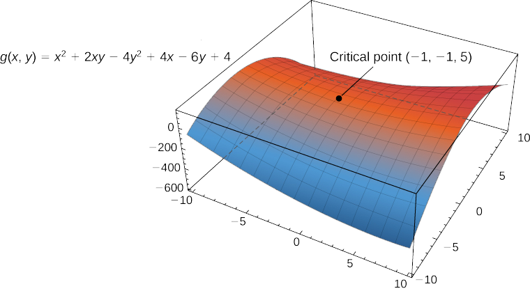
- \(g(x,y)=x^2+2xy−4y^2+4x−6y+4\)
Solution
a. First, we calculate \(f_x(x,y) \; \text{and} \; f_y(x,y):\)
\[\begin{align*} f_x(x,y) &=\dfrac{1}{2}(−18x+36)(4y^2−9x^2+24y+36x+36)^{−1/2} \\[4pt] &=\dfrac{−9x+18}{\sqrt{4y^2−9x^2+24y+36x+36}} \end{align*}\]
\[\begin{align*} f_y(x,y) &=\dfrac{1}{2}(8y+24)(4y^2−9x^2+24y+36x+36)^{−1/2} \\[4pt] &=\dfrac{4y+12}{\sqrt{4y^2−9x^2+24y+36x+36}} \end{align*}. \nonumber \]
Next, we set each of these expressions equal to zero:
\[\begin{align*} \dfrac{−9x+18}{\sqrt{4y^2−9x^2+24y+36x+36}} &=0 \\[4pt] \dfrac{4y+12}{\sqrt{4y^2−9x^2+24y+36x+36}} &=0. \end{align*}\]
Then, multiply each equation by its common denominator:
\[\begin{align*} −9x+18 &=0 \\[4pt] 4y+12 &=0. \end{align*}\]
Therefore, \(x=2\) and \(y=−3,\) so \((2,−3)\) is a critical point of \(f\).
We must also check for the possibility that the denominator of each partial derivative can equal zero, thus causing the partial derivative not to exist. Since the denominator is the same in each partial derivative, we need only do this once:
\[4y^2−9x^2+24y+36x+36=0. \label{critical1} \]
Equation \ref{critical1} represents a hyperbola. We should also note that the domain of \(f\) consists of points satisfying the inequality
\[4y^2−9x^2+24y+36x+36≥0. \nonumber \]
Therefore, any points on the hyperbola are not only critical points, they are also on the boundary of the domain. To put the hyperbola in standard form, we use the method of completing the square:
\[\begin{align*} 4y^2−9x^2+24y+36x+36 &=0 \\[4pt] 4y^2−9x^2+24y+36x &=−36 \\[4pt] 4y^2+24y−9x^2+36x &=−36 \\[4pt] 4(y^2+6y)−9(x^2−4x) &=−36 \\[4pt] 4(y^2+6y+9)−9(x^2−4x+4) &=−36−36+36 \\[4pt] 4(y+3)^2−9(x−2)^2 &=−36.\end{align*}\]
Dividing both sides by \(−36\) puts the equation in standard form:
\[\begin{align*} \dfrac{4(y+3)^2}{−36}−\dfrac{9(x−2)^2}{−36} &=1 \\[4pt] \dfrac{(x−2)^2}{4}−\dfrac{(y+3)^2}{9} &=1. \end{align*}\]
Notice that point \((2,−3)\) is the center of the hyperbola.
Thus, the critical points of the function \(f\) are \( (2, -3) \) and all points on the hyperbola, \(\dfrac{(x−2)^2}{4}−\dfrac{(y+3)^2}{9}=1\).
b. First, we calculate \(g_x(x,y)\) and \(g_y(x,y)\):
\[\begin{align*} g_x(x,y) &=2x+2y+4 \\[4pt] g_y(x,y) &=2x−8y−6. \end{align*}\]
Next, we set each of these expressions equal to zero, which gives a system of equations in \(x\) and \(y\):
\[\begin{align*} 2x+2y+4 &=0 \\[4pt] 2x−8y−6 &=0. \end{align*}\]
Subtracting the second equation from the first gives \(10y+10=0\), so \(y=−1\). Substituting this into the first equation gives \(2x+2(−1)+4=0\), so \(x=−1\).
Therefore \((−1,−1)\) is a critical point of \(g\). There are no points in \(\mathbb{R}^2\) that make either partial derivative not exist.
Figure \(\PageIndex{1}\) shows the behavior of the surface at the critical point.
Find the critical point of the function \(f(x,y)=x^3+2xy−2x−4y.\)
- Hint
-
Calculate \(f_x(x,y)\) and \(f_y(x,y)\), then set them equal to zero.
- Answer
-
The only critical point of \(f\) is \((2,−5)\).
The main purpose for determining critical points is to locate relative maxima and minima, as in single-variable calculus. When working with a function of one variable, the definition of a local extremum involves finding an interval around the critical point such that the function value is either greater than or less than all the other function values in that interval. When working with a function of two or more variables, we work with an open disk around the point.
Let \(z=f(x,y)\) be a function of two variables that is defined and continuous on an open set containing the point \((x_0,y_0).\) Then \(f\) has a local maximum at \((x_0,y_0)\) if
\[f(x_0,y_0)≥f(x,y) \nonumber \]
for all points \((x,y)\) within some disk centered at \((x_0,y_0)\). The number \(f(x_0,y_0)\) is called a local maximum value. If the preceding inequality holds for every point \((x,y)\) in the domain of \(f\), then \(f\) has a global maximum (also called an absolute maximum) at \((x_0,y_0).\)
The function \(f\) has a local minimum at \((x_0,y_0)\) if
\[f(x_0,y_0)≤f(x,y) \nonumber \]
for all points \((x,y)\) within some disk centered at \((x_0,y_0)\). The number \(f(x_0,y_0)\) is called a local minimum value. If the preceding inequality holds for every point \((x,y)\) in the domain of \(f\), then \(f\) has a global minimum (also called an absolute minimum) at \((x_0,y_0)\).
If \(f(x_0,y_0)\) is either a local maximum or local minimum value, then it is called a local extremum (see the following figure).
In Calculus 1, we showed that extrema of functions of one variable occur at critical points. The same is true for functions of more than one variable, as stated in the following theorem.
Let \(z=f(x,y)\) be a function of two variables that is defined and continuous on an open set containing the point \((x_0,y_0)\). Suppose \(f_x\) and \(f_y\) each exist at \((x_0,y_0)\). If f has a local extremum at \((x_0,y_0)\), then \((x_0,y_0)\) is a critical point of \(f\).
Second Derivative Test
Consider the function \(f(x)=x^3.\) This function has a critical point at \(x=0\), since \(f'(0)=3(0)^2=0\). However, \(f\) does not have an extreme value at \(x=0\). Therefore, the existence of a critical value at \(x=x_0\) does not guarantee a local extremum at \(x=x_0\). The same is true for a function of two or more variables. One way this can happen is at a saddle point. An example of a saddle point appears in the following figure.
Figure \(\PageIndex{3}\): Graph of the function \(z=x^2−y^2\). This graph has a saddle point at the origin.
In this graph, the origin is a saddle point. This is because the first partial derivatives of f\((x,y)=x^2−y^2\) are both equal to zero at this point, but it is neither a maximum nor a minimum for the function. Furthermore the vertical trace corresponding to \(y=0\) is \(z=x^2\) (a parabola opening upward), but the vertical trace corresponding to \(x=0\) is \(z=−y^2\) (a parabola opening downward). Therefore, it is both a global maximum for one trace and a global minimum for another.
Given the function \(z=f(x,y),\) the point \(\big(x_0,y_0,f(x_0,y_0)\big)\) is a saddle point if both \(f_x(x_0,y_0)=0\) and \(f_y(x_0,y_0)=0\), but \(f\) does not have a local extremum at \((x_0,y_0).\)
The second derivative test for a function of one variable provides a method for determining whether an extremum occurs at a critical point of a function. When extending this result to a function of two variables, an issue arises related to the fact that there are, in fact, four different second-order partial derivatives, although equality of mixed partials reduces this to three. The second derivative test for a function of two variables, stated in the following theorem, uses a discriminant \(D\) that replaces \(f''(x_0)\) in the second derivative test for a function of one variable.
Let \(z=f(x,y)\) be a function of two variables for which the first- and second-order partial derivatives are continuous on some disk containing the point \((x_0,y_0)\). Suppose \(f_x(x_0,y_0)=0\) and \(f_y(x_0,y_0)=0.\) Define the quantity
\[D=f_{xx}(x_0,y_0)f_{yy}(x_0,y_0)−\big(f_{xy}(x_0,y_0)\big)^2. \nonumber \]
Then:
- If \(D>0\) and \(f_{xx}(x_0,y_0)>0\), then f has a local minimum at \((x_0,y_0)\).
- If \(D>0\) and \(f_{xx}(x_0,y_0)<0\), then f has a local maximum at \((x_0,y_0)\).
- If \(D<0\), then \(f\) has a saddle point at \((x_0,y_0)\).
- If \(D=0\), then the test is inconclusive.
See Figure \(\PageIndex{4}\).

To apply the second derivative test, it is necessary that we first find the critical points of the function. There are several steps involved in the entire procedure, which are outlined in a problem-solving strategy.
Let \(z=f(x,y)\) be a function of two variables for which the first- and second-order partial derivatives are continuous on some disk containing the point \((x_0,y_0).\) To apply the second derivative test to find local extrema, use the following steps:
- Determine the critical points \((x_0,y_0)\) of the function \(f\) where \(f_x(x_0,y_0)=f_y(x_0,y_0)=0.\) Discard any points where at least one of the partial derivatives does not exist.
- Calculate the discriminant \(D=f_{xx}(x_0,y_0)f_{yy}(x_0,y_0)−\big(f_{xy}(x_0,y_0)\big)^2\) for each critical point of \(f\).
- Apply the four cases of the test to determine whether each critical point is a local maximum, local minimum, or saddle point, or whether the theorem is inconclusive.
Find the critical points for each of the following functions, and use the second derivative test to find the local extrema:
- \(f(x,y)=4x^2+9y^2+8x−36y+24\)
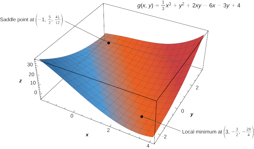
- \(g(x,y)=\dfrac{1}{3}x^3+y^2+2xy−6x−3y+4\)
Solution
a. Step 1 of the problem-solving strategy involves finding the critical points of \(f\). To do this, we first calculate \(f_x(x,y)\) and \(f_y(x,y)\), then set each of them equal to zero:
\[\begin{align*} f_x(x,y) &=8x+8 \\[4pt] f_y(x,y) &=18y−36. \end{align*}\]
Setting them equal to zero yields the system of equations
\[\begin{align*} 8x+8 &=0 \\[4pt] 18y−36 &=0. \end{align*}\]
The solution to this system is \(x=−1\) and \(y=2\). Therefore \((−1,2)\) is a critical point of \(f\).
Step 2 of the problem-solving strategy involves calculating \(D.\) To do this, we first calculate the second partial derivatives of \(f:\)
\[\begin{align*} f_{xx}(x,y) &=8 \\[4pt] f_{xy}(x,y) &=0 \\[4pt] f_{yy}(x,y) &=18. \end{align*}\]
Therefore, \(D=f_{xx}(−1,2)f_{yy}(−1,2)−\big(f_{xy}(−1,2)\big)^2=(8)(18)−(0)^2=144.\)
Step 3 states to apply the four cases of the test to classify the function's behavior at this critical point.
Since \(D>0\) and \(f_{xx}(−1,2)>0,\) this corresponds to case 1. Therefore, \(f\) has a local minimum at \((−1,2)\) as shown in the following figure.
Figure \(\PageIndex{5}\): The function \(f(x,y)\) has a local minimum at \((−1,2,−16).\) Note the scale on the \(y\)-axis in this plot is in thousands.
b. For step 1, we first calculate \(g_x(x,y)\) and \(g_y(x,y)\), then set each of them equal to zero:
\[\begin{align*} g_x(x,y) &=x^2+2y−6 \\[4pt] g_y(x,y) &=2y+2x−3. \end{align*}\]
Setting them equal to zero yields the system of equations
\[\begin{align*} x^2+2y−6 &=0 \\[4pt] 2y+2x−3 &=0. \end{align*}\]
To solve this system, first solve the second equation for \(y\). This gives \(y=\dfrac{3−2x}{2}\). Substituting this into the first equation gives
\[\begin{align*} x^2+3−2x−6 &=0 \\[4pt] x^2−2x−3 &=0 \\[4pt] (x−3)(x+1) &=0. \end{align*}\]
Therefore, \(x=−1\) or \(x=3\). Substituting these values into the equation \(y=\dfrac{3−2x}{2}\) yields the critical points \(\left(−1,\frac{5}{2}\right)\) and \(\left(3,−\frac{3}{2}\right)\).
Step 2 involves calculating the second partial derivatives of \(g\):
\[\begin{align*} g_{xx}(x,y) &=2x \\[4pt] g_{xy}(x,y) &=2\\[4pt] g_{yy}(x,y) &=2. \end{align*}\]
Then, we find a general formula for \(D\):
\[\begin{align*} D(x_0, y_0) &=g_{xx}(x_0,y_0)g_{yy}(x_0,y_0)−\big(g_{xy}(x_0,y_0)\big)^2 \\[4pt] &=(2x_0)(2)−2^2\\[4pt] &=4x_0−4.\end{align*}\]
Next, we substitute each critical point into this formula:
\[\begin{align*} D\left(−1,\tfrac{5}{2}\right) &=(2(−1))(2)−(2)^2=−4−4=−8 \\[4pt] D\left(3,−\tfrac{3}{2}\right) &=(2(3))(2)−(2)^2=12−4=8. \end{align*}\]
In step 3, we note that, applying Note to point \(\left(−1,\frac{5}{2}\right)\) leads to case \(3\), which means that \(\left(−1,\frac{5}{2}\right)\) is a saddle point. Applying the theorem to point \(\left(3,−\frac{3}{2}\right)\) leads to case \(1\), which means that \(\left(3,−\frac{3}{2}\right)\) corresponds to a local minimum as shown in the following figure.
Use the second derivative test to find the local extrema of the function
\[ f(x,y)=x^3+2xy−6x−4y^2. \nonumber \]
- Hint
-
Follow the problem-solving strategy for applying the second derivative test.
- Answer
-
\(\left(\frac{4}{3},\frac{1}{3}\right)\) is a saddle point, \(\left(−\frac{3}{2},−\frac{3}{8}\right)\) is a local maximum.
Absolute Maxima and Minima
When finding global extrema of functions of one variable on a closed interval, we start by checking the critical values over that interval and then evaluate the function at the endpoints of the interval. When working with a function of two variables, the closed interval is replaced by a closed, bounded set. A set is bounded if all the points in that set can be contained within a ball (or disk) of finite radius. First, we need to find the critical points inside the set and calculate the corresponding critical values. Then, it is necessary to find the maximum and minimum value of the function on the boundary of the set. When we have all these values, the largest function value corresponds to the global maximum and the smallest function value corresponds to the absolute minimum. First, however, we need to be assured that such values exist. The following theorem does this.
A continuous function \(f(x,y)\) on a closed and bounded set \(D\) in the plane attains an absolute maximum value at some point of \(D\) and an absolute minimum value at some point of \(D\).
Now that we know any continuous function \(f\) defined on a closed, bounded set attains its extreme values, we need to know how to find them.
Assume \(z=f(x,y)\) is a differentiable function of two variables defined on a closed, bounded set \(D\). Then \(f\) will attain the absolute maximum value and the absolute minimum value, which are, respectively, the largest and smallest values found among the following:
- The values of \(f\) at the critical points of \(f\) in \(D\).
- The values of \(f\) on the boundary of \(D\).
The proof of this theorem is a direct consequence of the extreme value theorem and Fermat’s theorem. In particular, if either extremum is not located on the boundary of \(D\), then it is located at an interior point of \(D\). But an interior point \((x_0,y_0)\) of \(D\) that’s an absolute extremum is also a local extremum; hence, \((x_0,y_0)\) is a critical point of \(f\) by Fermat’s theorem. Therefore the only possible values for the global extrema of \(f\) on \(D\) are the extreme values of \(f\) on the interior or boundary of \(D\).
Let \(z=f(x,y)\) be a continuous function of two variables defined on a closed, bounded set \(D\), and assume \(f\) is differentiable on \(D\). To find the absolute maximum and minimum values of \(f\) on \(D\), do the following:
- Determine the critical points of \(f\) in \(D\).
- Calculate \(f\) at each of these critical points.
- Determine the maximum and minimum values of \(f\) on the boundary of its domain.
- The maximum and minimum values of \(f\) will occur at one of the values obtained in steps \(2\) and \(3\).
Finding the maximum and minimum values of \(f\) on the boundary of \(D\) can be challenging. If the boundary is a rectangle or set of straight lines, then it is possible to parameterize the line segments and determine the maxima on each of these segments, as seen in Example \(\PageIndex{3}\). The same approach can be used for other shapes such as circles and ellipses.
If the boundary of the set \(D\) is a more complicated curve defined by a function \(g(x,y)=c\) for some constant \(c\), and the first-order partial derivatives of \(g\) exist, then the method of Lagrange multipliers can prove useful for determining the extrema of \(f\) on the boundary which is introduced in Lagrange Multipliers.
Use the problem-solving strategy for finding absolute extrema of a function to determine the absolute extrema of each of the following functions:
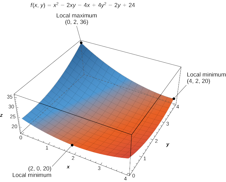
- \(f(x,y)=x^2−2xy+4y^2−4x−2y+24\) on the domain defined by \(0≤x≤4\) and \(0≤y≤2\)
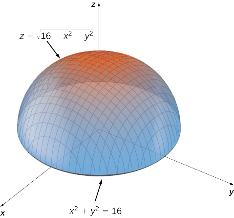
- \(g(x,y)=x^2+y^2+4x−6y\) on the domain defined by \(x^2+y^2≤16\)
Solution
a. Using the problem-solving strategy, step \(1\) involves finding the critical points of \(f\) on its domain. Therefore, we first calculate \(f_x(x,y)\) and \(f_y(x,y)\), then set them each equal to zero:
\[\begin{align*} f_x(x,y) &=2x−2y−4 \\[4pt] f_y(x,y) &=−2x+8y−2. \end{align*}\]
Setting them equal to zero yields the system of equations
\[\begin{align*} 2x−2y−4 &=0\\[4pt] −2x+8y−2 &=0. \end{align*}\]
The solution to this system is \(x=3\) and \(y=1\). Therefore \((3,1)\) is a critical point of \(f\). Calculating \(f(3,1)\) gives \(f(3,1)=17.\)
The next step involves finding the extrema of \(f\) on the boundary of its domain. The boundary of its domain consists of four line segments as shown in the following graph:
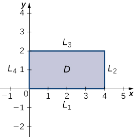
\(L_1\) is the line segment connecting \((0,0)\) and \((4,0)\), and it can be parameterized by the equations \(x(t)=t,y(t)=0\) for \(0≤t≤4\). Define \(g(t)=f\big(x(t),y(t)\big)\). This gives \(g(t)=t^2−4t+24\). Differentiating \(g\) leads to \(g′(t)=2t−4.\) Therefore, \(g\) has a critical value at \(t=2\), which corresponds to the point \((2,0)\). Calculating \(f(2,0)\) gives the \(z\)-value \(20\).
\(L_2\) is the line segment connecting \((4,0)\) and \((4,2)\), and it can be parameterized by the equations \(x(t)=4,y(t)=t\) for \(0≤t≤2.\) Again, define \(g(t)=f\big(x(t),y(t)\big).\) This gives \(g(t)=4t^2−10t+24.\) Then, \(g′(t)=8t−10\). g has a critical value at \(t=\frac{5}{4}\), which corresponds to the point \(\left(4,\frac{5}{4}\right).\) Calculating \(f\left(4,\frac{5}{4}\right)\) gives the \(z\)-value \(17.75\).
\(L_3\) is the line segment connecting \((0,2)\) and \((4,2)\), and it can be parameterized by the equations \(x(t)=t,y(t)=2\) for \(0≤t≤4.\) Again, define \(g(t)=f\big(x(t),y(t)\big).\) This gives \(g(t)=t^2−8t+36.\) The critical value corresponds to the point \((4,2).\) So, calculating \(f(4,2)\) gives the \(z\)-value \(20\).
\(L_4\) is the line segment connecting \((0,0)\) and \((0,2)\), and it can be parameterized by the equations \(x(t)=0,y(t)=t\) for \(0≤t≤2.\) This time, \(g(t)=4t^2−2t+24\) and the critical value \(t=\frac{1}{4}\) correspond to the point \(\left(0,\frac{1}{4}\right)\). Calculating \(f\left(0,\frac{1}{4}\right)\) gives the \(z\)-value \(23.75.\)
We also need to find the values of \(f(x,y)\) at the corners of its domain. These corners are located at \((0,0),(4,0),(4,2)\) and \((0,2)\):
\[\begin{align*} f(0,0) &=(0)^2−2(0)(0)+4(0)^2−4(0)−2(0)+24=24 \\[4pt] f(4,0) &=(4)^2−2(4)(0)+4(0)^2−4(4)−2(0)+24=24 \\[4pt] f(4,2) &=(4)^2−2(4)(2)+4(2)^2−4(4)−2(2)+24=20\\[4pt] f(0,2) &=(0)^2−2(0)(2)+4(2)^2−4(0)−2(2)+24=36. \end{align*}\]
The absolute maximum value is \(36\), which occurs at \((0,2)\), and the global minimum value is \(20\), which occurs at both \((4,2)\) and \((2,0)\) as shown in the following figure.
b. Using the problem-solving strategy, step \(1\) involves finding the critical points of \(g\) on its domain. Therefore, we first calculate \(g_x(x,y)\) and \(g_y(x,y)\), then set them each equal to zero:
\[\begin{align*} g_x(x,y) &=2x+4 \\[4pt] g_y(x,y) &=2y−6. \end{align*}\]
Setting them equal to zero yields the system of equations
\[\begin{align*} 2x+4 &=0 \\[4pt] 2y−6 &=0. \end{align*}\]
The solution to this system is \(x=−2\) and \(y=3\). Therefore, \((−2,3)\) is a critical point of \(g\). Calculating \(g(−2,3),\) we get
\[g(−2,3)=(−2)^2+3^2+4(−2)−6(3)=4+9−8−18=−13. \nonumber \]
The next step involves finding the extrema of g on the boundary of its domain. The boundary of its domain consists of a circle of radius \(4\) centered at the origin as shown in the following graph.
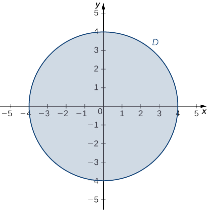
The boundary of the domain of \(g\) can be parameterized using the functions \(x(t)=4\cos t,\, y(t)=4\sin t\) for \(0≤t≤2π\). Define \(h(t)=g\big(x(t),y(t)\big):\)
\[\begin{align*} h(t) &=g\big(x(t),y(t)\big) \\[4pt] &=(4\cos t)^2+(4\sin t)^2+4(4\cos t)−6(4\sin t) \\[4pt] &=16\cos^2t+16\sin^2t+16\cos t−24\sin t\\[4pt] &=16+16\cos t−24\sin t. \end{align*}\]
Setting \(h′(t)=0\) leads to
\[\begin{align*} −16\sin t−24\cos t &=0 \\[4pt] −16\sin t &=24\cos t\\[4pt] \dfrac{−16\sin t}{−16\cos t} &=\dfrac{24\cos t}{−16\cos t} \\[4pt] \tan t &=−\dfrac{3}{2}. \end{align*}\]
This equation has two solutions over the interval \(0≤t≤2π\). One is \(t=π−\arctan (\frac{3}{2})\) and the other is \(t=2π−\arctan (\frac{3}{2})\). For the first angle,
\[\begin{align*} \sin t &=\sin(π−\arctan(\tfrac{3}{2}))=\sin (\arctan (\tfrac{3}{2}))=\dfrac{3\sqrt{13}}{13} \\[4pt] \cos t &=\cos (π−\arctan (\tfrac{3}{2}))=−\cos (\arctan (\tfrac{3}{2}))=−\dfrac{2\sqrt{13}}{13}. \end{align*}\]
Therefore, \(x(t)=4\cos t =−\frac{8\sqrt{13}}{13}\) and \(y(t)=4\sin t=\frac{12\sqrt{13}}{13}\), so \(\left(−\frac{8\sqrt{13}}{13},\frac{12\sqrt{13}}{13}\right)\) is a critical point on the boundary and
\[\begin{align*} g\left(−\tfrac{8\sqrt{13}}{13},\tfrac{12\sqrt{13}}{13}\right) &=\left(−\tfrac{8\sqrt{13}}{13}\right)^2+\left(\tfrac{12\sqrt{13}}{13}\right)^2+4\left(−\tfrac{8\sqrt{13}}{13}\right)−6\left(\tfrac{12\sqrt{13}}{13}\right) \\[4pt] &=\frac{144}{13}+\frac{64}{13}−\frac{32\sqrt{13}}{13}−\frac{72\sqrt{13}}{13} \\[4pt] &=\frac{208−104\sqrt{13}}{13}≈−12.844. \end{align*}\]
For the second angle,
\[\begin{align*} \sin t &=\sin (2π−\arctan (\tfrac{3}{2}))=−\sin (\arctan (\tfrac{3}{2}))=−\dfrac{3\sqrt{13}}{13} \\[4pt] \cos t &=\cos (2π−\arctan (\tfrac{3}{2}))=\cos (\arctan (\tfrac{3}{2}))=\dfrac{2\sqrt{13}}{13}. \end{align*}\]
Therefore, \(x(t)=4\cos t=\frac{8\sqrt{13}}{13}\) and \(y(t)=4\sin t=−\frac{12\sqrt{13}}{13}\), so \(\left(\frac{8\sqrt{13}}{13},−\frac{12\sqrt{13}}{13}\right)\) is a critical point on the boundary and
\[\begin{align*} g\left(\tfrac{8\sqrt{13}}{13},−\tfrac{12\sqrt{13}}{13}\right) &=\left(\tfrac{8\sqrt{13}}{13}\right)^2+\left(−\tfrac{12\sqrt{13}}{13}\right)^2+4\left(\tfrac{8\sqrt{13}}{13}\right)−6\left(−\tfrac{12\sqrt{13}}{13}\right) \\[4pt] &=\dfrac{144}{13}+\dfrac{64}{13}+\dfrac{32\sqrt{13}}{13}+\dfrac{72\sqrt{13}}{13}\\[4pt] &=\dfrac{208+104\sqrt{13}}{13}≈44.844. \end{align*}\]
The absolute minimum of \(g\) is \(−13,\) which is attained at the point \((−2,3)\), which is an interior point of \(D\). The absolute maximum of \(g\) is approximately equal to 44.844, which is attained at the boundary point \(\left(\frac{8\sqrt{13}}{13},−\frac{12\sqrt{13}}{13}\right)\). These are the absolute extrema of \(g\) on \(D\) as shown in the following figure.
Use the problem-solving strategy for finding absolute extrema of a function to find the absolute extrema of the function
\[f(x,y)=4x^2−2xy+6y^2−8x+2y+3 \nonumber \]
on the domain defined by \(0≤x≤2\) and \(−1≤y≤3.\)
- Hint
-
Calculate \(f_x(x,y)\) and \(f_y(x,y)\), and set them equal to zero. Then, calculate \(f\) for each critical point and find the extrema of \(f\) on the boundary of \(D\).
- Answer
-
The absolute minimum occurs at \((1,0): f(1,0)=−1.\)
The absolute maximum occurs at \((0,3): f(0,3)=63.\)
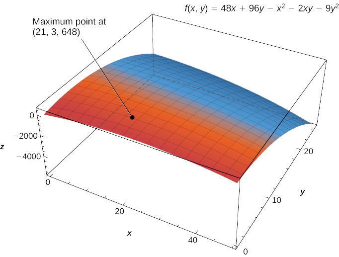
Pro-\(T\) company has developed a profit model that depends on the number \(x\) of golf balls sold per month (measured in thousands), and the number of hours per month of advertising \(y\), according to the function
\[ z=f(x,y)=48x+96y−x^2−2xy−9y^2, \nonumber \]
where \(z\) is measured in thousands of dollars. The maximum number of golf balls that can be produced and sold is \(50,000\), and the maximum number of hours of advertising that can be purchased is \(25\). Find the values of \(x\) and \(y\) that maximize profit, and find the maximum profit.
Solution
Using the problem-solving strategy, step \(1\) involves finding the critical points of \(f\) on its domain. Therefore, we first calculate \(f_x(x,y)\) and \(f_y(x,y),\) then set them each equal to zero:
\[\begin{align*} f_x(x,y) &=48−2x−2y \\[4pt] f_y(x,y) &=96−2x−18y. \end{align*}\]
Setting them equal to zero yields the system of equations
\[\begin{align*} 48−2x−2y &=0 \\[4pt] 96−2x−18y &=0. \end{align*}\]
The solution to this system is \(x=21\) and \(y=3\). Therefore \((21,3)\) is a critical point of \(f\). Calculating \(f(21,3)\) gives \(f(21,3)=48(21)+96(3)−21^2−2(21)(3)−9(3)^2=648.\)
The domain of this function is \(0≤x≤50\) and \(0≤y≤25\) as shown in the following graph.
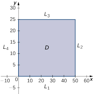
\(L_1\) is the line segment connecting \((0,0)\) and \((50,0),\) and it can be parameterized by the equations \(x(t)=t,y(t)=0\) for \(0≤t≤50.\) We then define \(g(t)=f(x(t),y(t)):\)
\[\begin{align*} g(t) &=f(x(t),y(t)) \\[4pt] &=f(t,0)\\[4pt] &=48t+96(0)−y^2−2(t)(0)−9(0)^2\\[4pt] &=48t−t^2. \end{align*}\]
Setting \(g′(t)=0\) yields the critical point \(t=24,\) which corresponds to the point \((24,0)\) in the domain of \(f\). Calculating \(f(24,0)\) gives \(576.\)
\(L_2\) is the line segment connecting \((50,0)\) and \((50,25)\), and it can be parameterized by the equations \(x(t)=50,y(t)=t\) for \(0≤t≤25\). Once again, we define \(g(t)=f\big(x(t),y(t)\big):\)
\[\begin{align*} g(t) &=f\big(x(t),y(t)\big)\\[4pt] &=f(50,t)\\[4pt] &=48(50)+96t−50^2−2(50)t−9t^2 \\[4pt] &=−9t^2−4t−100. \end{align*}\]
This function has a critical point at \(t =−\frac{2}{9}\), which corresponds to the point \((50,−29)\). This point is not in the domain of \(f\).
\(L_3\) is the line segment connecting \((0,25)\) and \((50,25)\), and it can be parameterized by the equations \(x(t)=t,y(t)=25\) for \(0≤t≤50\). We define \(g(t)=f\big(x(t),y(t)\big)\):
\[\begin{align*} g(t) &=f\big(x(t),y(t)\big)\\[4pt] &=f(t,25) \\[4pt] &=48t+96(25)−t^2−2t(25)−9(25^2) \\[4pt] &=−t^2−2t−3225. \end{align*}\]
This function has a critical point at \(t=−1\), which corresponds to the point \((−1,25),\) which is not in the domain.
\(L_4\) is the line segment connecting \((0,0)\) to \((0,25)\), and it can be parameterized by the equations \(x(t)=0,y(t)=t\) for \(0≤t≤25\). We define \(g(t)=f\big(x(t),y(t)\big)\):
\[\begin{align*} g(t) &=f\big(x(t),y(t)\big) \\[4pt] &=f(0,t) \\[4pt] &=48(0)+96t−(0)^2−2(0)t−9t^2 \\[4pt] &=96t−9t^2. \end{align*}\]
This function has a critical point at \(t=\frac{16}{3}\), which corresponds to the point \(\left(0,\frac{16}{3}\right)\), which is on the boundary of the domain. Calculating \(f\left(0,\frac{16}{3}\right)\) gives \(256\).
We also need to find the values of \(f(x,y)\) at the corners of its domain. These corners are located at \((0,0),(50,0),(50,25)\) and \((0,25)\):
\[\begin{align*} f(0,0) &=48(0)+96(0)−(0)^2−2(0)(0)−9(0)^2=0\\[4pt] f(50,0) &=48(50)+96(0)−(50)^2−2(50)(0)−9(0)^2=−100 \\[4pt] f(50,25) &=48(50)+96(25)−(50)^2−2(50)(25)−9(25)^2=−5825 \\[4pt] f(0,25) &=48(0)+96(25)−(0)^2−2(0)(25)−9(25)^2=−3225. \end{align*}\]
The maximum value is \(648\), which occurs at \((21,3)\). Therefore, a maximum profit of \($648,000\) is realized when \(21,000\) golf balls are sold and \(3\) hours of advertising are purchased per month as shown in the following figure.
Key Concepts
- A critical point of the function \(f(x,y)\) is any point \((x_0,y_0)\) where either \(f_x(x_0,y_0)=f_y(x_0,y_0)=0\), or at least one of \(f_x(x_0,y_0)\) and \(f_y(x_0,y_0)\) do not exist.
- A saddle point is a point \((x_0,y_0)\) where \(f_x(x_0,y_0)=f_y(x_0,y_0)=0\), but \(f(x_0,y_0)\) is neither a maximum nor a minimum at that point.
- To find extrema of functions of two variables, first find the critical points, then calculate the discriminant and apply the second derivative test.
Key Equations
- Discriminant
\(D=f_{xx}(x_0,y_0)f_{yy}(x_0,y_0)−(f_{xy}(x_0,y_0))^2\)
Glossary
- critical point of a function of two variables
-
the point \((x_0,y_0)\) is called a critical point of \(f(x,y)\) if one of the two following conditions holds:
1. \(f_x(x_0,y_0)=f_y(x_0,y_0)=0\)
2. At least one of \(f_x(x_0,y_0)\) and \(f_y(x_0,y_0)\) do not exist
- discriminant
- the discriminant of the function \(f(x,y)\) is given by the formula \(D=f_{xx}(x_0,y_0)f_{yy}(x_0,y_0)−(f_{xy}(x_0,y_0))^2\)
- saddle point
- given the function \(z=f(x,y),\) the point \((x_0,y_0,f(x_0,y_0))\) is a saddle point if both \(f_x(x_0,y_0)=0\) and \(f_y(x_0,y_0)=0\), but \(f\) does not have a local extremum at \((x_0,y_0)\)