2.2E: Exercises for Section 2.2
- Page ID
- 49549
Intuitive Definition of Limits
For exercises 1 - 2, consider the function \(f(x)=\dfrac{x^2−1}{|x−1|}\).
1) [T] Complete the following table for the function. Round your solutions to four decimal places.
| \(x\) | \(f(x)\) | \(x\) | \(f(x)\) |
|---|---|---|---|
| 0.9 | a. | 1.1 | e. |
| 0.99 | b. | 1.01 | f. |
| 0.999 | c. | 1.001 | g. |
| 0.9999 | d. | 1.0001 | h. |
2) What do your results in the preceding exercise indicate about the two-sided limit \(\displaystyle \lim_{x→1}f(x)\)? Explain your response.
- Answer
-
\(\displaystyle \lim_{x \to 1}f(x)\) does not exist because \(\displaystyle \lim_{x \to 1^−}f(x)=−2≠\lim_{x \to 1^+}f(x)=2\).
For exercises 3 - 5, consider the function \(f(x)=(1+x)^{1/x}\).
3) [T] Make a table showing the values of \(f\) for \(x=−0.01,\;−0.001,\;−0.0001,\;−0.00001\) and for \(x=0.01,\;0.001,\;0.0001,\;0.00001\). Round your solutions to five decimal places.
| \(x\) | \(f(x)\) | \(x\) | \(f(x)\) |
|---|---|---|---|
| -0.01 | a. | 0.01 | e. |
| -0.001 | b. | 0.001 | f. |
| -0.0001 | c. | 0.0001 | g. |
| -0.00001 | d. | 0.00001 | h. |
4) What does the table of values in the preceding exercise indicate about the function \(f(x)=(1+x)^{1/x}\)?
- Answer
- \(\displaystyle \lim_{x \to 0}(1+x)^{1/x}\approx 2.7183\).
5) To which mathematical constant do the values in the preceding exercise appear to be approaching? This is the actual limit here.
In exercises 6 - 8, use the given values to set up a table to evaluate the limits. Round your solutions to eight decimal places.
6) [T] \(\displaystyle \lim_{x \to 0}\frac{\sin 2x}{x};\quad ±0.1,\; ±0.01, \; ±0.001, \;±.0001\)
| \(x\) | \(\frac{\sin 2x}{x}\) | \(x\) | \(\frac{\sin 2x}{x}\) |
|---|---|---|---|
| -0.1 | a. | 0.1 | e. |
| -0.01 | b. | 0.01 | f. |
| -0.001 | c. | 0.001 | g. |
| -0.0001 | d. | 0.0001 | h. |
- Answer
- a. 1.98669331; b. 1.99986667; c. 1.99999867; d. 1.99999999; e. 1.98669331; f. 1.99986667; g. 1.99999867; h. 1.99999999;
\(\displaystyle \lim_{x \to 0}\frac{\sin 2x}{x}=2\)
7) [T] \(\displaystyle \lim_{x \to 0}\frac{\sin 3x}{x} ±0.1, \; ±0.01, \; ±0.001, \; ±0.0001\)
| \(x\) | \(\frac{\sin 3x}{x}\) | \(x\) | \(\frac{\sin 3x}{x}\) |
|---|---|---|---|
| -0.1 | a. | 0.1 | e. |
| -0.01 | b. | 0.01 | f. |
| -0.001 | c. | 0.001 | g. |
| -0.0001 | d. | 0.0001 | h. |
8) Use the preceding two exercises to conjecture (guess) the value of the following limit: \(\displaystyle \lim_{x \to 0}\frac{\sin ax}{x}\) for \(a\), a positive real value.
- Answer
- \(\displaystyle \lim_{x \to 0}\frac{\sin ax}{x}=a\)
[T] In exercises 9 - 14, set up a table of values to find the indicated limit. Round to eight significant digits.
9) \(\displaystyle \lim_{x \to 2}\frac{x^2−4}{x^2+x−6}\)
| \(x\) | \(\frac{x^2−4}{x^2+x−6}\) | \(x\) | \(\frac{x^2−4}{x^2+x−6}\) |
|---|---|---|---|
| 1.9 | a. | 2.1 | e. |
| 1.99 | b. | 2.01 | f. |
| 1.999 | c. | 2.001 | g. |
| 1.9999 | d. | 2.0001 | h. |
10) \(\displaystyle \lim_{x \to 1}(1−2x)\)
| \(x\) | \(1−2x\) | \(x\) | \(1−2x\) |
|---|---|---|---|
| 0.9 | a. | 1.1 | e. |
| 0.99 | b. | 1.01 | f. |
| 0.999 | c. | 1.001 | g. |
| 0.9999 | d. | 1.0001 | h. |
- Answer
- a. −0.80000000; b. −0.98000000; c. −0.99800000; d. −0.99980000; e. −1.2000000; f. −1.0200000; g. −1.0020000; h. −1.0002000;
\( \displaystyle \lim_{x \to 1}(1−2x)=−1\)
11) \(\displaystyle \lim_{x \to 0}\frac{5}{1−e^{1/x}}\)
| \(x\) | \(\frac{5}{1−e^{1/x}}\) | \(x\) | \(\frac{5}{1−e^{1/x}}\) |
|---|---|---|---|
| -0.1 | a. | 0.1 | e. |
| -0.01 | b. | 0.01 | f. |
| -0.001 | c. | 0.001 | g. |
| -0.0001 | d. | 0.0001 | h. |
12) \(\displaystyle \lim_{z \to 0}\frac{z−1}{z^2(z+3)}\)
| \(z\) | \(\frac{z−1}{z^2(z+3)}\) | \(z\) | \(\frac{z−1}{z^2(z+3)}\) |
|---|---|---|---|
| -0.1 | a. | 0.1 | e. |
| -0.01 | b. | 0.01 | f. |
| -0.001 | c. | 0.001 | g. |
| -0.0001 | d. | 0.0001 | h. |
- Answer
- a. −37.931034; b. −3377.9264; c. −333,777.93; d. −33,337,778; e. −29.032258; f. −3289.0365; g. −332,889.04; h. −33,328,889
\( \displaystyle \lim_{x \to 0}\frac{z−1}{z^2(z+3)}=−∞\)
13) \(\displaystyle \lim_{t \to 0^+}\frac{\cos t}{t}\)
| \(t\) | \(\frac{\cos t}{t}\) |
|---|---|
| 0.1 | a. |
| 0.01 | b. |
| 0.001 | c. |
| 0.0001 | d. |
14) \(\displaystyle \lim_{x \to 2}\frac{1−\frac{2}{x}}{x^2−4}\)
| \(x\) | \(\frac{1−\frac{2}{x}}{x^2−4}\) | \(x\) | \(\frac{1−\frac{2}{x}}{x^2−4}\) |
|---|---|---|---|
| 1.9 | a. | 2.1 | e. |
| 1.99 | b. | 2.01 | f. |
| 1.999 | c. | 2.001 | g. |
| 1.9999 | d. | 2.0001 | h. |
- Answer
- a. 0.13495277; b. 0.12594300; c. 0.12509381; d. 0.12500938; e. 0.11614402; f. 0.12406794; g. 0.12490631; h. 0.12499063;
\( \displaystyle ∴\lim_{x \to 2}\frac{1−\frac{2}{x}}{x^2−4}=0.1250=\frac{1}{8}\)
[T] In exercises 15 - 16, set up a table of values and round to eight significant digits. Based on the table of values, make a guess about what the limit is. Then, use a calculator to graph the function and determine the limit. Was the conjecture correct? If not, why does the method of tables fail?
15) \(\displaystyle \lim_{θ \to 0}\sin\left(\frac{π}{θ}\right)\)
| \(θ\) | \(\sin\left(\frac{π}{θ}\right)\) | \(θ\) | \(\sin\left(\frac{π}{θ}\right)\) |
|---|---|---|---|
| -0.1 | a. | 0.1 | e. |
| -0.01 | b. | 0.01 | f. |
| -0.001 | c. | 0.001 | g. |
| -0.0001 | d. | 0.0001 | h. |
16) \(\displaystyle \lim_{α \to 0^+} \frac{1}{α}\cos\left(\frac{π}{α}\right)\)
| \(a\) | \(\frac{1}{α}\cos\left(\frac{π}{α}\right)\) |
|---|---|
| 0.1 | a. |
| 0.01 | b. |
| 0.001 | c. |
| 0.0001 | d. |
- Answer
-
a. 10.00000; b. 100.00000; c. 1000.0000; d. 10,000.000;
Guess: \(\displaystyle \lim_{α→0^+}\frac{1}{α}\cos\left(\frac{π}{α}\right)=∞\);
Actual: DNE , since the graph shows the function oscillates wildly between values approaching positive infinity and values approaching negative infinity, as the value of \(α\) approaches \(0\) from the positive side.![A graph of the function (1/alpha) * cos (pi / alpha), which oscillates gently until the interval [-.2, .2], where it oscillates rapidly, going to infinity and negative infinity as it approaches the y axis.](https://math.libretexts.org/@api/deki/files/1863/CNX_Calc_Figure_02_02_214.jpeg?revision=1&size=bestfit&width=417&height=348)
In exercises 17 - 20, consider the graph of the function\(y=f(x)\) shown here. Which of the statements about \(y=f(x)\) are true and which are false? Explain why a statement is false.
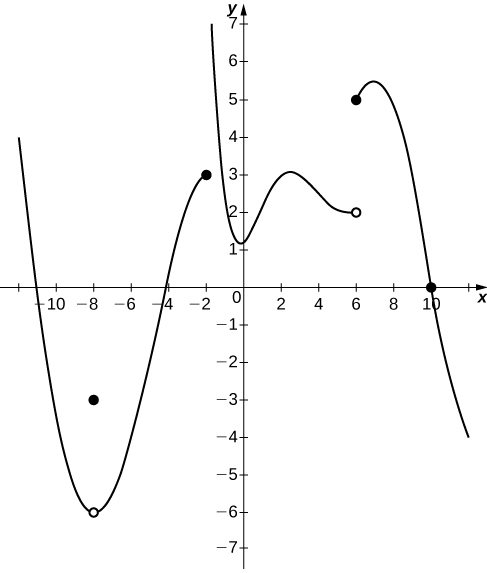
17) \(\displaystyle \lim_{x→10}f(x)=0\)
18) \(\displaystyle \lim_{x→−2^+}f(x)=3\)
- Answer
- False; \(\displaystyle \lim_{x→−2^+}f(x)=+∞\)
19) \(\displaystyle \lim_{x→−8}f(x)=f(−8)\)
20) \(\displaystyle \lim_{x→6}f(x)=5\)
- Answer
- False; \(\displaystyle \lim_{x→6}f(x)\) DNE since \(\displaystyle \lim_{x→6^−}f(x)=2\) and \(\displaystyle \lim_{x→6^+}f(x)=5\).
In exercises 21 - 25, use the following graph of the function \(y=f(x)\) to find the values, if possible. Estimate when necessary.
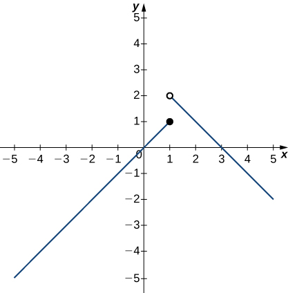
21) \(\displaystyle \lim_{x→1^−}f(x)\)
22) \(\displaystyle \lim_{x→1^+}f(x)\)
- Answer
- \(2\)
23) \(\displaystyle \lim_{x→1}f(x)\)
24) \(\displaystyle \lim_{x→2}f(x)\)
- Answer
- \(1\)
25) \(f(1)\)
In exercises 26 - 29, use the graph of the function \(y=f(x)\) shown here to find the values, if possible. Estimate when necessary.
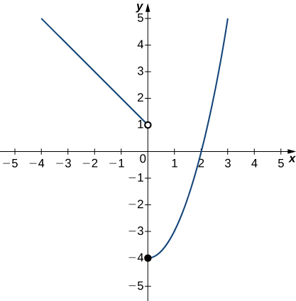
26) \(\displaystyle \lim_{x→0^−}f(x)\)
- Answer
- \(1\)
27) \(\displaystyle \lim_{x→0^+}f(x)\)
28) \(\displaystyle \lim_{x→0}f(x)\)
- Answer
- DNE
29) \(\displaystyle \lim_{x→2}f(x)\)
In exercises 30 - 35, use the graph of the function \(y=f(x)\) shown here to find the values, if possible. Estimate when necessary.
![A graph of a piecewise function with three segments, all linear. The first exists for x < -2, has a slope of 1, and ends at the open circle at (-2, 0). The second exists over the interval [-2, 2], has a slope of -1, goes through the origin, and has closed circles at its endpoints (-2, 2) and (2,-2). The third exists for x>2, has a slope of 1, and begins at the open circle (2,2).](https://math.libretexts.org/@api/deki/files/1897/CNX_Calc_Figure_02_02_204.jpeg?revision=1&size=bestfit&width=417&height=424)
30) \(\displaystyle \lim_{x→−2^−}f(x)\)
- Answer
- \(0\)
31) \(\displaystyle \lim_{x→−2^+}f(x)\)
32) \(\displaystyle \lim_{x→−2}f(x)\)
- Answer
- DNE
33) \(\displaystyle \lim_{x→2^−}f(x)\)
34) \(\displaystyle \lim_{x→2^+}f(x)\)
- Answer
- \(2\)
35) \(\displaystyle \lim_{x→2}f(x)\)
In exercises 36 - 38, use the graph of the function \(y=g(x)\) shown here to find the values, if possible. Estimate when necessary.
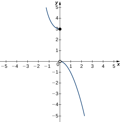
36) \(\displaystyle \lim_{x→0^−}g(x)\)
- Answer
- \(3\)
37) \(\displaystyle \lim_{x→0^+}g(x)\)
38) \(\displaystyle \lim_{x→0}g(x)\)
- Answer
- DNE
In exercises 39 - 41, use the graph of the function \(y=h(x)\) shown here to find the values, if possible. Estimate when necessary.
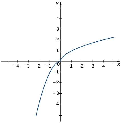
39) \(\displaystyle \lim_{x→0^−}h(x)\)
40) \(\displaystyle \lim_{x→0^+}h(x)\)
- Answer
- \(0\)
41) \(\displaystyle \lim_{x→0}h(x)\)
In exercises 42 - 46, use the graph of the function \(y=f(x)\) shown here to find the values, if possible. Estimate when necessary.
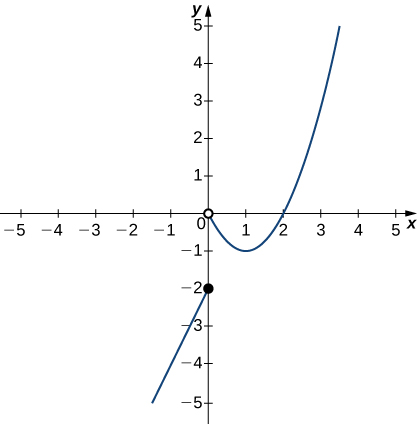
42) \(\displaystyle \lim_{x→0^−}f(x)\)
- Answer
- \(-2\)
43) \(\displaystyle \lim_{x→0^+}f(x)\)
44) \(\displaystyle \lim_{x→0}f(x)\)
- Answer
- DNE
45) \(\displaystyle \lim_{x→1}f(x)\)
46) \(\displaystyle \lim_{x→2}f(x)\)
- Answer
- \(0\)
Infinite Limits
In exercises 47 - 51, sketch the graph of a function with the given properties.
47) \(\displaystyle \lim_{x→2}f(x)=1, \quad \lim_{x→4^−}f(x)=3, \quad \lim_{x→4^+}f(x)=6, \quad x=4\) is not defined.
48) \(\displaystyle \lim_{x→−∞}f(x)=0, \quad \lim_{x→−1^−}f(x)=−∞, \quad \lim_{x→−1^+}f(x)=∞,\quad \lim_{x→0}f(x)=f(0), \quad f(0)=1, \quad \lim_{x→∞}f(x)=−∞\)
- Answer
-
Answers may vary
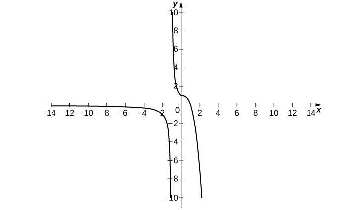
49) \(\displaystyle \lim_{x→−∞}f(x)=2, \quad \lim_{x→3^−}f(x)=−∞, \quad \lim_{x→3^+}f(x)=∞, \quad \lim_{x→∞}f(x)=2, \quad f(0)=-\frac{1}{3}\)
50) \(\displaystyle \lim_{x→−∞}f(x)=2,\quad \lim_{x→−2}f(x)=−∞,\quad \lim_{x→∞}f(x)=2,\quad f(0)=0\)
- Answer
-
Answer may vary
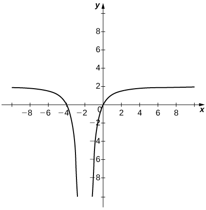
51) \(\displaystyle \lim_{x→−∞}f(x)=0,\quad \lim_{x→−1^−}f(x)=∞,\quad \lim_{x→−1^+}f(x)=−∞, \quad f(0)=−1, \quad \lim_{x→1^−}f(x)=−∞, \quad \lim_{x→1^+}f(x)=∞, \quad \lim_{x→∞}f(x)=0\)
52) Shock waves arise in many physical applications, ranging from supernovas to detonation waves. A graph of the density of a shock wave with respect to distance, \(x\), is shown here. We are mainly interested in the location of the front of the shock, labeled \(X_{SF}\) in the diagram.
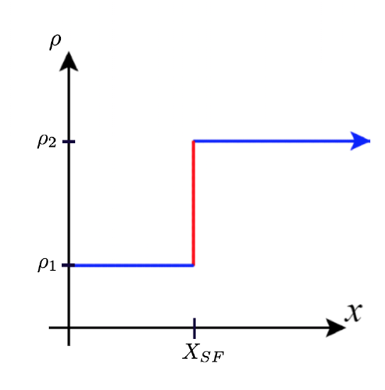
a. Evaluate \(\displaystyle \lim_{x→X_{SF}^+}ρ(x)\).
b. Evaluate \(\displaystyle \lim_{x→X_{SF}^−}ρ(x)\).
c. Evaluate \(\displaystyle \lim_{x→X_{SF}}ρ(x)\). Explain the physical meanings behind your answers.
- Answer
- a. \(ρ_2\) b. \(ρ_1\) c. DNE unless \(ρ_1=ρ_2\). As you approach \(X_{SF}\) from the right, you are in the high-density area of the shock. When you approach from the left, you have not experienced the “shock” yet and are at a lower density.
53) A track coach uses a camera with a fast shutter to estimate the position of a runner with respect to time. A table of the values of position of the athlete versus time is given here, where \(x\) is the position in meters of the runner and \(t\) is time in seconds. What is \(\displaystyle \lim_{t→2}x(t)\)? What does it mean physically?
| \(t(sec)\) | \(x(m)\) |
|---|---|
| 1.75 | 4.5 |
| 1.95 | 6.1 |
| 1.99 | 6.42 |
| 2.01 | 6.58 |
| 2.05 | 6.9 |
| 2.25 | 8.5 |


