2.5: The Riemann Hypothesis

Definition 2.19

The Riemann zeta function \(\zeta(z)\) is a complex function defined as follows on \(\{z \in \mathbb{C} | \mbox{Re}z > 1\}\)

\[\zeta (z) = \sum_{n=1}^{\infty} n^{-z} \nonumber\]

On other values of \(z \in \mathbb{C}\) it is defined by the analytic continuation of this function (except at \(z = 1\) where it has a simple pole).

Analytic continuation is akin to replacing \(e^x\) where \(x\) is real by \(e^z\) where \(z\) is complex. Another example is the series \(\sum_{j=0}^{\infty} z^j\). This series diverges for \(|z| > 1\). But as an analytic function, it can be replaced by \((1-z)^{-1}\) on all of \(\mathbb{C}\) except at the pole \(z = 1\) where it diverges.

Recall that an analytic function is a function that is differentiable. Equivalently, it is a function that is locally given by a convergent power series. If \(f\) and \(g\) are two analytic continuations to a region \(U\) of a function \(h\) given on a region \(V \subset U\), then the difference \(f-g\) is zero on some \(U\) and therefore all its power expansions are zero and so it must be zero on the the entire region. Hence, analytic conjugations are unique. That is the reason they are meaningful. For more details, see for example [4, 14].

It is customary to denote the argument of the zeta function by \(s\). We will do so from here on out. Note that \(|n-s| = n-\mbox{Re} s\), and so for \(\mbox{Re} s > 1\) the series is absolutely convergent. At this point, the student should remember – or look up in [23] – the fact that absolutely convergent series can be rearranged arbitrarily without changing the sum. This leads to the following proposition.

Proposition 2.20

For \(\mbox{Re} s > 1\) we have

\[\sum_{n=1}^{\infty} n-s = \prod_{p prime} (1-p^{-s})^{-1} \nonumber\]

There are two common proofs of this formula. It is worth presenting both.

Proof

The first proof uses the Fundamental Theorem of Arithmetic. First, we recall that use geometric series

\[(1-p^{-s})^{-1} = \sum_{k=0}^{\infty} p^{-ks} \nonumber\]

to rewrite the right hand of the Euler product. This gives

\[\prod_{p prime} (1-p^{-s})^{-1} = (\sum_{k_1 = 0}^{\infty} p_{1}^{-k_{1}s}) (\sum_{k_2 = 0}^{\infty} p_{2}^{-k_{2}s}) (\sum_{k_3 = 0}^{\infty} p_{3}^{-k_{3}s}) \nonumber\]

Re-arranging terms yields

\[\dots = (p_{1}^{k_{1}}p_{2}^{k_{2}}p_{3}^{k_{3}} \dots)^{-s} \nonumber\]

By the Fundamental Theorem of Arithmetic, the expression \((p_{1}^{k_{1}}p_{2}^{k_{2}}p_{3}^{k_{3}} \dots)\) runs through all positive integers exactly once. Thus upon re-arranging again we obtain the left hand of Euler’s formula.

The second proof, the one that Euler used, employs a sieve method. This time, we start with the left hand of the Euler product. If we multiply \(\zeta\) by \(2^{-s}\), we get back precisely the terms with \(n\) even. So

\[(1-2^{-s}) \zeta(s) = 1+3^{-s}+5^{-s}+\cdots = \sum_{2 \nmid n} n^{-s} \nonumber\]

Subsequently we multiply this expression by \((1-3^{-s})\). This has the effect of removing the terms that remain where \(n\) is a multiple of \(3\). It follows that eventually

\[(1-p_{l}^{-s}) \dots (1-p_{1}^{-s}) \zeta (s) = \sum_{p_{1} \nmid n, \cdots p_{l} \nmid n} n^{-s} \nonumber\]

The argument used in Eratosthenes sieve (Section 1.1) now serves to show that in the right hand side of the last equation all terms other than \(1\) disappear as l tends to infinity. Therefore, the left hand tends to 1, which implies the proposition.

The most important theorem concerning primes is probably the following (without proof).

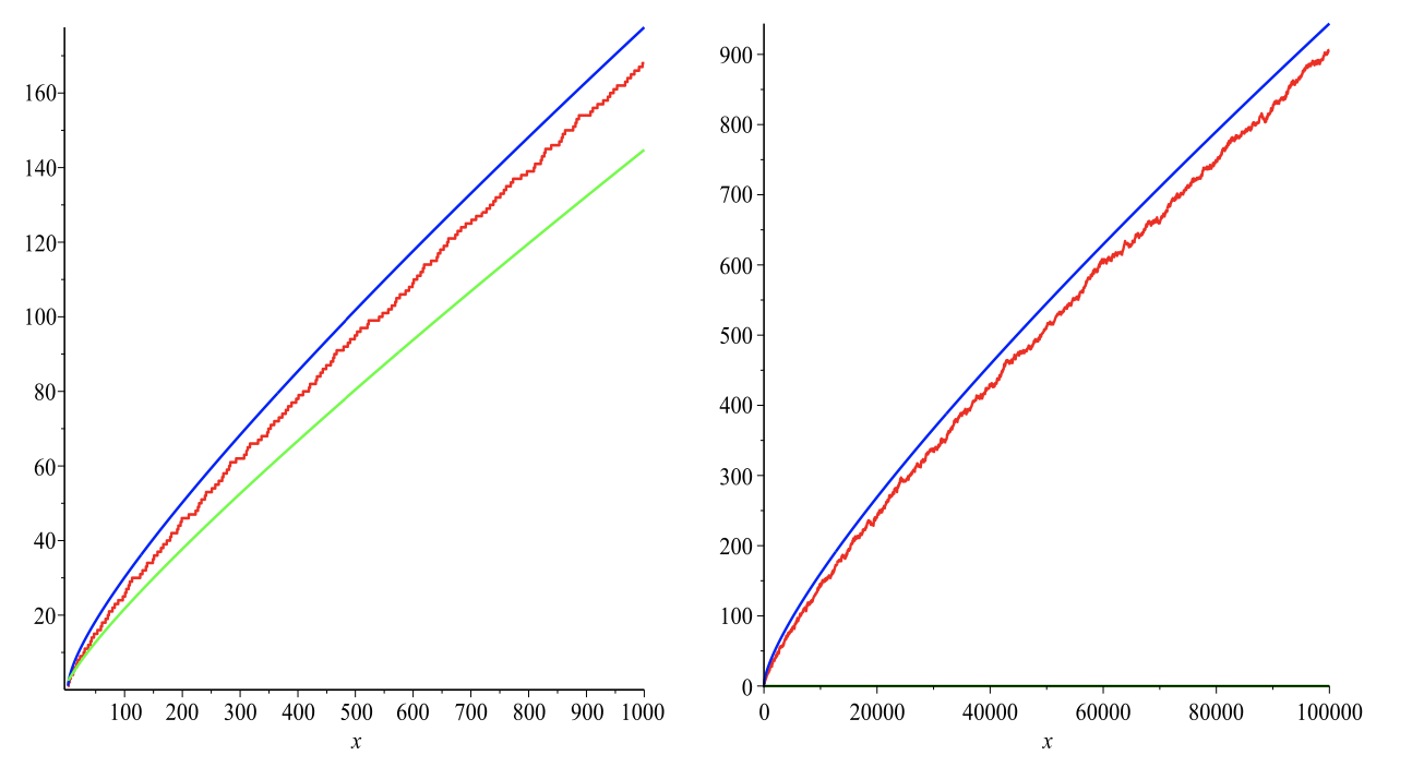
Figure 3. On the left, the function \(\int_{2}^{x} \mbox{ln} t dt\) in blue, \(\pi (x)\) in red, and \(x/ \mbox{ln}x\) in green. On the right, we have \(\int_{2}^{x} \mbox{ln} t dt - x/\mbox{ln} x\) in blue, \(\pi (x)- x/\mbox{ln} x\) in red.

Theorem 2.21 (Prime Number Theorem)

Let \(\pi (x)\) denote the prime counting function, that is: the number of primes less than or equal to \(x > 2\).

Then

1. \(\lim_{x \rightarrow \infty} \frac{\pi (x)}{(x/\mbox{ln} x)} = 1\) and
2. \(\lim_{x \rightarrow \infty} \frac{\pi (x)}{\int_{2}^{x} \mbox{ln} t dt} = 1\)

where \(\mbox{ln}\) is the natural logarithm.

The first estimate is the easier one to prove, the second is the more accurate one. In Figure 3 on the left, we plotted, for \(x \in [2,1000]\), from top to bottom the functions \(\int_{2}^{x} \mbox{ln} t dt\) in blue, \(\pi (x)\) in red, and \(x/\mbox{ln} x\). In the right hand figure, we augment the domain to \(x \in [2, 100000]\). and plot the difference of these functions with \(x/\mbox{ln} x\). It now becomes clear that \(\int_{2}^{x} \mbox{ln} t dt\) is indeed a much better approximation of \(\pi (x)\). From this figure one may be tempted to conclude that \(\int_{2}^{x} \mbox{ln} t dt - \pi (x)\) is always greater than or equal to zero. This, however, is false. It is known that there are infinitely many n for which \(\int_{2}^{x} \mbox{ln} t dt - \pi (x) < 0\). The first such \(n\) is called the Skewes number. Not much is known about this number, except that it is less than 10317.

Perhaps the most important open problem in all of mathematics is the following. It concerns the analytic continuation of \(\zeta (s)\) given above.

Conjecture 2.22 (Riemann Hypothesis)

All non-real zeros of \(\zeta (s)\) lie on the line \(\mbox{Re} s = \frac{1}{2}\)

In his only paper on number theory [20], Riemann realized that the hypothesis enabled him to describe detailed properties of the distribution of primes in terms of of the location of the non-real zero of \(\zeta (s)\). This completely unexpected connection between so disparate fields – analytic functions and primes in \(\mathbb{N}-\)spoke to the imagination and led to an enormous interest in the subject. In further research, it has been shown that the hypothesis is also related to other areas of mathematics, such as, for example, the spacings between eigenvalues of random Hermitian matrices [2], and even physics [5, 6].