3.1: The Euclidean Algorithm

Last updated
Save as PDF

Page ID: 60308

$ \newcommand{\vecs}[1]{\overset { \scriptstyle \rightharpoonup} {\mathbf{#1}} } $ $ \newcommand{\vecd}[1]{\overset{-\!-\!\rightharpoonup}{\vphantom{a}\smash {#1}}} $$\newcommand{\id}{\mathrm{id}}$ $ \newcommand{\Span}{\mathrm{span}}$ $ \newcommand{\kernel}{\mathrm{null}\,}$ $ \newcommand{\range}{\mathrm{range}\,}$ $ \newcommand{\RealPart}{\mathrm{Re}}$ $ \newcommand{\ImaginaryPart}{\mathrm{Im}}$ $ \newcommand{\Argument}{\mathrm{Arg}}$ $ \newcommand{\norm}[1]{\| #1 \|}$ $ \newcommand{\inner}[2]{\langle #1, #2 \rangle}$ $ \newcommand{\Span}{\mathrm{span}}$ $\newcommand{\id}{\mathrm{id}}$ $ \newcommand{\Span}{\mathrm{span}}$ $ \newcommand{\kernel}{\mathrm{null}\,}$ $ \newcommand{\range}{\mathrm{range}\,}$ $ \newcommand{\RealPart}{\mathrm{Re}}$ $ \newcommand{\ImaginaryPart}{\mathrm{Im}}$ $ \newcommand{\Argument}{\mathrm{Arg}}$ $ \newcommand{\norm}[1]{\| #1 \|}$ $ \newcommand{\inner}[2]{\langle #1, #2 \rangle}$ $ \newcommand{\Span}{\mathrm{span}}$$\newcommand{\AA}{\unicode[.8,0]{x212B}}$

Lemma 3.1

In the division algorithm of Definition2.4, we have $\gcd(r_{1},r_{2}) = \gcd(r_{2}, r_{3})$.

Proof: On the one hand, we have $r_{1} = r_{2}q_{2}+r_{3}$, and so any common divisor of $r_{2}$ and $r_{3}$ must also be a divisor of $r_{1}$ (and of $r_{2}$). Vice versa, since $r_{1}-r_{2}q_{2} = r_{3}$, we have that any common divisor of $r_{1}$ and $r_{2}$ must also be a divisor of $r_{3}$ (and of $r_{2}$).

Thus by calculating $r_{3}$, the residue of $r_{1}$ modulo $r_{2}$, we have simplified the computation of $\gcd (r_{1}, r_{2})$. This is because $r_{3}$ is strictly smaller (in absolute value) than both $r_{1}$ and $r_{2}$. In turn, the computation of $\gcd (r_{2}, r_{3})$ can be simplified similarly, and so the process can be repeated. Since the $r_{i}$ form a monotone decreasing sequence in $\mathbb{N}$, this process must end when $r_{n}+1 = 0$ after a finite number of steps. We then have $gcd(r_{1},r_{2}) = gcd(r_{n},0) = r_{n}$.

Corollary 3.2

Given $r_{1} > r_{2} > 0$, apply the division algorithm until $r_{n} > r_{n+1} = 0$. Then $\gcd (r_{1}, r_{2}) = \gcd(r_{n}, 0) = r_{n}$. Since $r_{i}$ is decreasing, the algorithm always ends.

Definition 3.3

The repeated application of the division algorithm to compute $\gcd(r_{1}, r_{2})$ is called the Euclidean algorithm.

We now give a framework to reduce the messiness of these repeated computations. Suppose we want to compute $\gcd(188, 158)$. We do the following computations:

\[188 = 158·1+30 \nonumber\]

\[158 = 30·5+8 \nonumber\]

\[30 = 8·3+6 \nonumber\]

\[8 = 6·1+2 \nonumber\]

\[6 = 2·3+0 \nonumber\]

We see that $\gcd(188,158) = 2$. The numbers that multiply the $r_{i}$ are the quotients of the division algorithm (see the proof of Lemma 2.3). If we call them $q_{i-1}$, the computation looks as follows:

\[\begin{array} {c} {r_{1} = r_{2} q_{2}+r_{3}}\\ {r_{2} = r_{3} q_{3}+r_{4}}\\ {\vdots}\\ {r_{n-3} = r_{n-2} q_{n-2}+r_{n-3}}\\ {r_{n-2} = r_{n-1} q_{n-1}+r_{n-2}}\\ {r_{n-1} = r_{n} q_{n}+0} \end{array}\]

where we use the convention that $r_{n+1} = 0$ while $r_{n} \ne 0$. Observe that with that convention, (3.1) consists of $n-1$ steps. A much more concise form (in part based on a suggestion of Katahdin [16]) to render this computation is as follows.

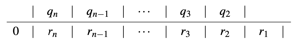
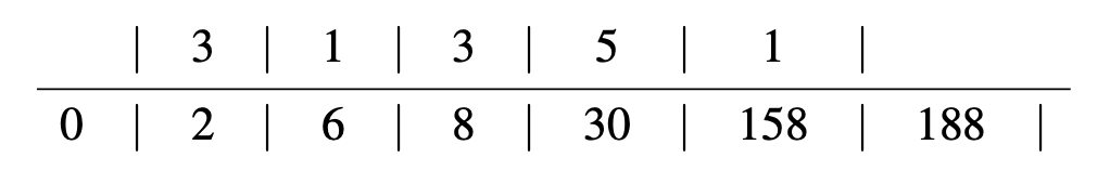
$Screen Shot 2021-04-21 at 3.48.54 PM.png$

Thus, each step $r_{i+1} |r_{i}|$ is similar to the usual long division, except that its quotient $q_{i+1}$ is placed above $r_{i+1}$ (and not above $r_{i}$), while its remainder $r_{i+2}$ is placed all the way to the left of of $r_{i+1}$. The example we worked out before now it looks like:

$Screen Shot 2021-04-21 at 3.50.42 PM.png$

There is a beautiful visualization of this process outlined in exercise 3.4.