
3.6: Catalan Numbers
- Page ID
- 7157

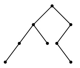
A rooted binary tree is a type of graph that is particularly of interest in some areas of computer science. A typical rooted binary tree is shown in Figure \(\PageIndex{1}\). The root is the topmost vertex. The vertices below a vertex and connected to it by an edge are the children of the vertex. It is a binary tree because all vertices have 0, 1, or 2 children. How many different rooted binary trees are there with \(n\) vertices?
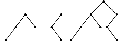
Let us denote this number by \(C_n\); these are the Catalan numbers. For convenience, we allow a rooted binary tree to be empty, and let \(C_0=1\). Then it is easy to see that \(C_1=1\) and \(C_2=2\), and not hard to see that \(C_3=5\). Notice that any rooted binary tree on at least one vertex can be viewed as two (possibly empty) binary trees joined into a new tree by introducing a new root vertex and making the children of this root the two roots of the original trees; see Figure \(\PageIndex{2}\). (To make the empty tree a child of the new vertex, simply do nothing, that is, omit the corresponding child.)
Thus, to make all possible binary trees with \(n\) vertices, we start with a root vertex, and then for its two children insert rooted binary trees on \(k\) and \(l\) vertices, with \(k+l=n-1\), for all possible choices of the smaller trees. Now we can write
\[ C_n=\sum_{i=0}^{n-1} C_iC_{n-i-1}. \nonumber \]
For example, since we know that \(C_0=C_1=1\) and \(C_2=2\),
\[ C_3 = C_0C_2 + C_1C_1+C_2C_0 = 1\cdot2 + 1\cdot1 + 2\cdot1 = 5, \nonumber \]
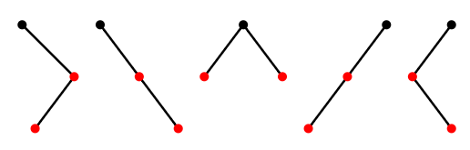
as mentioned above. Once we know the trees on 0, 1, and 2 vertices, we can combine them in all possible ways to list the trees on 3 vertices, as shown in Figure \(\PageIndex{3}\). Note that the first two trees have no left child, since the only tree on 0 vertices is empty, and likewise the last two have no right child.
Now we use a generating function to find a formula for \(C_n\). Let \(f=\sum_{i=0}^\infty C_ix^i\). Now consider \(f^2\): the coefficient of the term \(x^n\) in the expansion of \(f^2\) is \(\sum_{i=0}^{n} C_iC_{n-i}\), corresponding to all possible ways to multiply terms of \(f\) to get an \(x^n\) term: \[ C_0\cdot C_nx^n + C_1x\cdot C_{n-1}x^{n-1} + C_2x^2\cdot C_{n-2}x^{n-2} +\cdots+C_nx^n\cdot C_0. \nonumber\] Now we recognize this as precisely the sum that gives \(C_{n+1}\), so \(f^2 = \sum_{n=0}^\infty C_{n+1}x^n\). If we multiply this by \(x\) and add 1 (which is \(C_0\)) we get exactly \(f\) again, that is, \(xf^2+1=f\) or \(xf^2-f+1=0\); here 0 is the zero function, that is, \(xf^2-f+1\) is 0 for all x. Using the quadratic formula,
\[ f={1\pm\sqrt{1-4x}\over 2x}, \nonumber \]
as long as \(x\not=0\). It is not hard to see that as \(x\) approaches 0,
\[ {1+\sqrt{1-4x}\over 2x} \nonumber\]
goes to infinity while
\[ {1-\sqrt{1-4x}\over 2x}\nonumber \]
goes to 1. Since we know \(f(0)=C_0=1\), this is the \(f\) we want.
Now by Newton's Binomial Theorem, we can expand
\[ \sqrt{1-4x} = (1+(-4x))^{1/2} =\sum_{n=0}^\infty {1/2\choose n}(-4x)^n.\nonumber \]
Then
\[ {1-\sqrt{1-4x}\over 2x} = \sum_{n=1}^\infty -{1\over 2}{1/2\choose n}(-4)^nx^{n-1} = \sum_{n=0}^\infty -{1\over 2}{1/2\choose n+1}(-4)^{n+1}x^n. \nonumber \]
Expanding the binomial coefficient \(1/2\choose n+1\) and reorganizing the expression, we discover that
\[ C_n = -{1\over 2}{1/2\choose n+1}(-4)^{n+1} = {1\over n+1}{2n\choose n}.\nonumber \]
In Exercise 1.E.3.7 in Section 1.E, we saw that the number of properly matched sequences of parentheses of length \(2n\) is \({2n\choose n}-{2n\choose n+1}\), and called this \(C_n\). It is not difficult to see that
\[ {2n\choose n}-{2n\choose n+1}={1\over n+1}{2n\choose n},\nonumber \]
so the formulas are in agreement.
Temporarily let \(A_n\) be the number of properly matched sequences of parentheses of length \(2n\), so from the exercise we know \(A_n={2n\choose n}-{2n\choose n+1}\). It is possible to see directly that \(A_0=A_1=1\) and that the numbers \(A_n\) satisfy the same recurrence relation as do the \(C_n\), which implies that \(A_n=C_n\), without manipulating the generating function.
There are many counting problems whose answers turns out to be the Catalan numbers. Enumerative Combinatorics: Volume 2, by Richard Stanley, contains a large number of examples.