15.3: Map Colouring

Last updated
Save as PDF

Page ID: 60151

Joy Morris
University of Lethbridge

$ \newcommand{\vecs}[1]{\overset { \scriptstyle \rightharpoonup} {\mathbf{#1}} } $ $ \newcommand{\vecd}[1]{\overset{-\!-\!\rightharpoonup}{\vphantom{a}\smash {#1}}} $$\newcommand{\id}{\mathrm{id}}$ $ \newcommand{\Span}{\mathrm{span}}$ $ \newcommand{\kernel}{\mathrm{null}\,}$ $ \newcommand{\range}{\mathrm{range}\,}$ $ \newcommand{\RealPart}{\mathrm{Re}}$ $ \newcommand{\ImaginaryPart}{\mathrm{Im}}$ $ \newcommand{\Argument}{\mathrm{Arg}}$ $ \newcommand{\norm}[1]{\| #1 \|}$ $ \newcommand{\inner}[2]{\langle #1, #2 \rangle}$ $ \newcommand{\Span}{\mathrm{span}}$ $\newcommand{\id}{\mathrm{id}}$ $ \newcommand{\Span}{\mathrm{span}}$ $ \newcommand{\kernel}{\mathrm{null}\,}$ $ \newcommand{\range}{\mathrm{range}\,}$ $ \newcommand{\RealPart}{\mathrm{Re}}$ $ \newcommand{\ImaginaryPart}{\mathrm{Im}}$ $ \newcommand{\Argument}{\mathrm{Arg}}$ $ \newcommand{\norm}[1]{\| #1 \|}$ $ \newcommand{\inner}[2]{\langle #1, #2 \rangle}$ $ \newcommand{\Span}{\mathrm{span}}$$\newcommand{\AA}{\unicode[.8,0]{x212B}}$

Suppose we have a map of an island that has been divided into states.

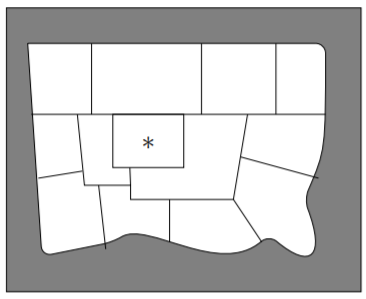
$clipboard_eba8864abf3246bcc6391879904aac345.png$

Traditionally, map-makers colour the different states so as to ensure that if two states share a border, they are not coloured with the same colour. (This makes it easier to distinguish the borders.) If two states simply meet at a corner, then they may be coloured with the same colour.

Using additional colours used to add to the cost of producing the map. Also, if there are too many colours they become harder and harder to distinguish amongst. The question is, without knowing in advance what the map will look like, is there a bound on how many colours will be required to colour it? If so, what is that bound? In other words, what is the largest number of colours that might be required to colour some map?

Well over a century ago, mathematicians observed that it never seemed to require more than $4$ colours to colour a map. The map shown above does require $4$ colours, since the central rectangular state (marked with an asterisk) and the three states that surround it must all receive different colours (each shares a border with each of the others). Unfortunately, they couldn’t prove that no more would ever be required, although a number of purported proofs were published and later found to have errors.

Although the bound of $4$ eluded many attempts at proof, in $1890$ Percy John Heawood successfully proved that $5$ colours suffice to colour any map. (His method was based on an incorrect proof of the Four Colour Theorem by Kempe, from $1879$.) This result is known as the Five Colour Theorem. Its proof is slightly technical but not difficult, and we will give it in a moment. First, we will give a very short proof that $6$ colours suffice.

Notice that if we turn the map into a graph by placing a vertex wherever borders meet, and an edge wherever there is a border, this problem is equivalent to finding a proper vertex colouring of the planar dual of this graph. Thus, what we will actually prove is that the vertices of any planar graph can be properly coloured using $6$ (or in the subsequent result, $5$) colours. There is a detail that we are skimming over here: the planar dual could have loops, which would make it impossible to colour the graph. However, this can only happen if there is a face of the original map that meets itself along a border, which would never happen in a map. The planar dual might also have multiedges, but this does not affect the number of colours required to properly colour the graph, so we can delete any multiedges and assume that we are dealing with a simple planar graph.

Proposition $\PageIndex{1}$

Every planar graph is properly $6$-colourable.

Proof

Towards a contradiction, suppose that there is a planar graph that is not properly $6$-colourable. By deleting edges and vertices, we can find a subgraph $G$ that is a $7$-critical planar graph.

By Corollary 15.2.3, we must have $δ(G) ≤ 5$ since $G$ is planar. But by Theorem 14.3.1, we must have

\[δ(G) ≥ 7 − 1 = 6\]

since $G$ is $7$-critical. This contradiction serves to prove that every planar graph is properly $6$-colourable.

Theorem $\PageIndex{1}$: Five Colour Theorem

Every planar graph is properly $5$-colourable.

Proof

Towards a contradiction, suppose that there is a planar graph that is not properly $5$-colourable. By deleting edges and vertices, we can find a subgraph $G$ that is a $6$-critical planar graph. Since $G$ is planar, Corollary 15.2.3 tells us that $δ(G) ≤ 5$. We also know from Theorem 14.3.1 that $δ(G) ≥ 6−1 = 5$ since $G$ is $6$-critical. Let v be a vertex of valency $δ(G) = 5$.

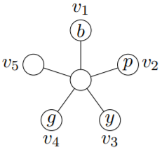
By the definition of a $k$-critical graph, $G \setminus \{v\}$ can be properly $5$-coloured. Since $G$ itself cannot be properly $5$-coloured, the neighbours of $v$ must all have been assigned different colours in the proper $5$-colouring of $G \setminus \{v\}$. Let’s label the neighbours of $v$ as $v_1$, $v_2$, $v_3$, $v_4$, and $v_5$ as they appear clockwise around $v$. We will call the colour of $v_1$ blue, the colour of $v_2$ purple, the colour of $v_3$ yellow, and the colour of $v_4$ green, as shown in the picture. Here is a picture (where, because this text is printed in black-and-white, we have put the first letter of a colour onto a vertex, instead of actually colouring the vertex).

$clipboard_ec6fe8f1ed3009fd368ca4b9b537dbb3f.png$

Consider the subgraph consisting of the vertices coloured blue or yellow (and all edges between such vertices). If $v_1$ and $v_3$ are not in the same connected component of this subgraph, then in the connected component that contains $v_1$, we could interchange the colours yellow and blue. Since we are doing this to everything in a connected component of the yellow-blue subgraph, the result will still be a proper colouring, but $v_1$ now has colour yellow, so $v$ can be coloured with blue. This contradicts the fact that $G$ is $6$-critical, so it must be the case that $v_1$ and $v_3$ are in the same connected component of the yellow-blue subgraph. In particular, there is a walk from $v_1$ to $v_3$ that uses only yellow and blue vertices. By Proposition 12.3.1, there is in fact a path from $v_1$ to $v_3$ that uses only yellow and blue vertices.

Similarly, if we consider the subgraph consisting of the vertices coloured purple or green (and all edges between such vertices), we see that there must be a path from $v_2$ to $v_4$ that uses only purple or green vertices.

There is no way to draw the yellow-blue path from $v_1$ to $v_3$ and the purple-green path from $v_2$ to $v_4$, without the two paths crossing each other. Since the graph is planar, they must cross each other at a vertex, $u$. Since $u$ is on the yellow-blue path, it must be coloured either yellow or blue. Since $u$ is on the purple-green path, it must be coloured either purple or green. It’s not possible to satisfy both of these conditions on the colour of $u$. This contradiction serves to prove that no planar $6$-critical graph exists, so every planar graph is properly $5$-colourable.

In fact, Appel and Haken proved the Four Colour Theorem in $1976$.

Theorem $\PageIndex{2}$: Four Colour Theorem

Every planar graph is properly $4$-colourable.

Proof

Their proof involved considering a very large number of cases – so many that they used a computer to analyse them all. Although computers are often used in mathematical work now, this was the first proof that could not reasonably be verified by hand. It was viewed with suspicion for a long time, but is now generally accepted.

One of the methods by which mathematicians attempted unsuccessfully to prove the Four Colour Theorem seemed particularly promising, and has led to a lot of interesting work in its own right. We require a couple of definitions to explain the connection.

Definition: Cubic Graph

A cubic graph is a graph for which all of the vertices have valency $3$.

Definition: Bridge

A bridge in a connected graph is an edge whose deletion disconnects the graph.

Theorem $\PageIndex{3}$

The problem of $4$-colouring a planar graph is equivalent to the problem of $3$-edge-colouring a cubic graph that has no bridges.

Proof

We’ll prove one direction of the equivalence stated in this theorem; the other direction is a bit more complicated.

Suppose that every planar graph can be properly $4$-coloured, and that $G$ is a (simple) bridgeless cubic graph, embedded in the plane. We’ll show that there is a proper $3$-edge-colouring of $G$. Since $G$ is bridgeless, we don’t run into the problem of a loop in the planar dual, so the Four Colour Theorem applies to the faces of $G$. Properly colour the faces of $G$ with colours red, green, yellow, and black. Every edge of $G$ lies between faces of two distinct colours, by the definition of a proper colouring of a map. Colour the edges of $G$ according to the following table: if the colours of the faces separated by the edge $e$ are the colours listed in the left-hand column, then use the colour listed in the right-hand column to colour $e$.

Face Colours	Edge Colour
green, black	dashed
yellow, black	dotted
red, black	solid
green, yellow	solid
green, red	dotted
red, yellow	dashed

Let $v$ be an arbitrary vertex. We will show that the three edges incident with $v$ must all receive different colours. Since $3$ edges meet at $v$, three faces also meet at $v$, and every pair of these faces share an edge. Thus the three faces that meet at $v$ must all receive different colours. There are four different cases, depending on which colour is not used for a face at $v$. We show what happens in the following picture, using $R$, $G$, $Y$, and $B$ to indicate the face colours, and colouring the edges according to the table above in each case.

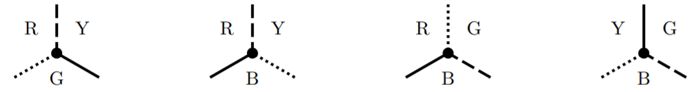
$clipboard_e21b16d747cb3169a8baa7bcf8f53c44c.png$

In each case, the three edges incident with $v$ are assigned different colours, so this is a proper $3$-edge colouring of $G$.

This theorem was proven by Tait in $1880$; he thought that every cubic graph with no bridges must be $3$-edge-colourable, and thus that he had proven the Four Colour Theorem. In fact, Vizing’s Theorem tells us that any cubic graph can be $4$-edge-coloured, so we would only need to reduce the number of colours by $1$ in order to prove the Four Colour Theorem. The problem, therefore, boils down to proving that there are no bridgeless planar cubic graphs that are class two.

In $1881$, Petersen published the Petersen graph that we saw previously in Example 14.3.4.

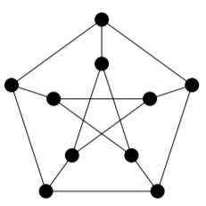
$clipboard_e344e5b311f3550ecaec3e214d2f339ba.png$

This graph is cubic and has no bridges, but is not $3$-edge-colourable (this can be proved using a case-by-case analysis). Thus, there exist bridgeless cubic graphs that are class two! Many people have tried to find other examples, as classifying these could provide a proof of the Four Colour Theorem.

For many years, Martin Gardner wrote a column in the Scientific American about interesting math problems and puzzles. As the Four Colour Theorem is easy to explain without technical language, it was a topic he wrote about. When writing about the importance of bridgeless cubic class two graphs, he decided they needed a more appealing name. Since they seemed rare and elusive, he called them snarks, after Lewis Carroll’s poem “The Hunting of the Snark.” The name has stuck.

Definition: Snark

A snark is a bridgeless cubic class two graph.

Two infinite families and a number of individual snarks are known. There is no reason to believe that these are all of the snarks that exist. By the Four Colour Theorem, we know that there are no planar snarks; if we could find a direct proof that there are no planar snarks, this would provide a new proof of the Four Colour Theorem.

Exercise $\PageIndex{1}$

1) Prove that if a cubic graph $G$ has a Hamilton cycle, then $G$ is a class one graph.

2) Properly $4$-colour the faces of the map given at the start of this section.

3) The map given at the start of this section can be made into a cubic graph, by placing a vertex everywhere two borders meet (including the coast as a border) and edges where there are borders. Use the method from the proof of Theorem 15.3.3 to properly $3$-edge-colour this cubic graph, using your $4$-colouring of the faces.

4) Prove that a graph $G$ that admits a planar embedding has an Euler tour if and only if every planar dual of $G$ is bipartite.

5) Prove that if a graph $G$ that admits a planar embedding in which every face is surrounded by exactly $3$ edges, $G$ is $3$-colourable if and only if it has an Euler tour.