
1.2: Basic Concepts
- Page ID
- 9391

A differential equation is an equation that contains one or more derivatives of an unknown function. The order of a differential equation is the order of the highest derivative that it contains. A differential equation is an ordinary differential equation if it involves an unknown function of only one variable, or a partial differential equation if it involves partial derivatives of a function of more than one variable. For now we’ll consider only ordinary differential equations, and we’ll just call them differential equations.
Throughout this text, all variables and constants are real unless it is stated otherwise. We’ll usually use \(x\) for the independent variable unless the independent variable is time; then we’ll use \(t\).
The simplest differential equations are first order equations of the form
\[{dy\over dx}=f(x) \nonumber\]
or equivalently
\[y'=f(x), \nonumber\]
where \(f\) is a known function of \(x\). We already know from calculus how to find functions that satisfy this kind of equation. For example, if
\[y'=x^3, \nonumber\]
then
\[y=\int x^3\, dx={x^4\over4}+c, \nonumber\]
where \(c\) is an arbitrary constant. If \(n>1\) we can find functions \(y\) that satisfy equations of the form
\[\label{eq:1.2.1} y^{(n)}=f(x)\]
by repeated integration. Again, this is a calculus problem.
Except for illustrative purposes in this section, there’s no need to consider differential equations like Equation \ref{eq:1.2.1}. We’ll usually consider differential equations that can be written as
\[\label{eq:1.2.2} y^{(n)}=f(x,y,y', \dots,y^{(n-1)}),\]
where at least one of the functions \(y\), \(y'\), …, \(y^{(n-1)}\) actually appears on the right. Here are some examples:
\begin{array}{rcll} {dy\over dx}-x^2&=&0&\mbox{ (first order)}, \\ {dy\over dx}+2xy^2&=&-2&\mbox{ (first order)}, \\ {d^2y\over dx^2}+2 {dy\over dx}+y&=&2x&\mbox{ (second order)}, \\ xy'''+y^2&=&\sin x &\mbox{ (third order)}, \\ y^{(n)}+xy'+3y&=&x&\mbox{ (n-th order)}. \nonumber \end{array}
Although none of these equations is written as in Equation \ref{eq:1.2.2}, all of them can be written in this form:
\[\begin{array}{rcl} y'&=&x^2, \\ y'&=&-2-2xy^2, \\ y''&=&2x-2y'-y, \\ y'''&=& \dfrac{\sin x-y^2}{x}, \\[4pt] y^{(n)}&=&x-xy'-3y. \end{array}\nonumber \]
Solutions of Differential Equations
A solution of a differential equation is a function that satisfies the differential equation on some open interval; thus, \(y\) is a solution of Equation \ref{eq:1.2.2} if \(y\) is \(n\) times differentiable and
\[y^{(n)}(x)=f(x,y(x),y'(x), \dots,y^{(n-1)}(x)) \nonumber\]
for all \(x\) in some open interval \((a,b)\). In this case, we also say that \(y\) is a solution of Equation \ref{eq:1.2.2} on \((a,b)\). Functions that satisfy a differential equation at isolated points are not interesting. For example, \(y=x^2\) satisfies
\[xy'+x^2=3x \nonumber\]
if and only if \(x=0\) or \(x=1\), but it is not a solution of this differential equation because it does not satisfy the equation on an open interval.
The graph of a solution of a differential equation is a solution curve. More generally, a curve \(C\) is said to be an integral curve of a differential equation if every function \(y=y(x)\) whose graph is a segment of \(C\) is a solution of the differential equation. Thus, any solution curve of a differential equation is an integral curve, but an integral curve need not be a solution curve.
If \(a\) is any positive constant, the circle
\[\label{eq:1.2.3} x^2+y^2=a^2\]
is an integral curve of
\[\label{eq:1.2.4} y'=-{x\over y}.\]
Solution
To see this, note that the only functions whose graphs are segments of Equation \ref{eq:1.2.3} are
\[y_1=\sqrt{a^2-x^2} \quad \text{and} \quad y_2=-\sqrt{a^2-x^2}.\nonumber \]
We leave it to you to verify that these functions both satisfy Equation \ref{eq:1.2.4} on the open interval \((-a,a)\). However, Equation \ref{eq:1.2.3} is not a solution curve of Equation \ref{eq:1.2.4}, since it is not the graph of a function.
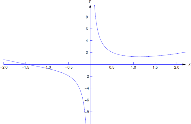
Verify that
\[\label{eq:1.2.5} y={x^2\over3}+{1\over x}\]
is a solution of
\[\label{eq:1.2.6} xy'+y=x^2\]
on \((0,\infty)\) and on \((-\infty,0)\).
Solution
Substituting Equation \ref{eq:1.2.5} and
\[y'={2x\over3} - {1\over x^2}\nonumber \]
into Equation \ref{eq:1.2.6} yields
\[xy'(x)+y(x)=x \left({2x\over3} - {1\over x^2}\right)+ \left({x^2\over3}+{1\over x}\right)=x^2\nonumber \]
for all \(x\ne0\). Therefore \(y\) is a solution of Equation \ref{eq:1.2.6} on \((-\infty,0)\) and \((0,\infty)\). However, \(y\) isn’t a solution of the differential equation on any open interval that contains \(x=0\), since \(y\) is not defined at \(x=0\).
Figure 1.2.2 shows the graph of Equation \ref{eq:1.2.5}. The part of the graph of Equation \ref{eq:1.2.5} on \((0,\infty)\) is a solution curve of Equation \ref{eq:1.2.6}, as is the part of the graph on \((-\infty,0)\).
Show that if \(c_1\) and \(c_2\) are constants then
\[\label{eq:1.2.7} y=(c_1+c_2x)e^{-x}+2x-4\]
is a solution of \[\label{eq:1.2.8} y''+2y'+y=2x\] on \((-\infty,\infty)\).
Solution
Differentiating Equation \ref{eq:1.2.7} twice yields
\[y'=-(c_1+c_2x)e^{-x}+c_2e^{-x}+2 \nonumber\]
and
\[y''=(c_1+c_2x)e^{-x}-2c_2e^{-x}, \nonumber\]
so
\[\begin{align*} y''+2y'+y&=(c_1+c_2x)e^{-x}-2c_2e^{-x} + 2\left[-(c_1+c_2x)e^{-x}+c_2e^{-x}+2\right] +(c_1+c_2x)e^{-x}+2x-4 \\[4pt] &=(1-2+1)(c_1+c_2x)e^{-x}+(-2+2)c_2e^{-x} + 4+2x-4 \\[4pt] &=2x \end{align*}\]
for all values of \(x\). Therefore \(y\) is a solution of Equation \ref{eq:1.2.8} on \((-\infty,\infty)\).
Find all solutions of
\[\label{eq:1.2.9} y^{(n)}=e^{2x}.\]
Solution
Integrating Equation \ref{eq:1.2.9} yields
\[y^{(n-1)}={e^{2x}\over2}+k_1, \nonumber\]
where \(k_1\) is a constant. If \(n\ge2\), integrating again yields
\[y^{(n-2)}={e^{2x}\over4}+k_1x+k_2. \nonumber\]
If \(n\ge3\), repeatedly integrating yields
\[\label{eq:1.2.10} y={e^{2x}\over2^n}+k_1{x^{n-1}\over (n-1)!}+k_2{x^{n-2}\over (n-2)!}+\cdots+k_n,\]
where \(k_1\), \(k_2\), …, \(k_n\) are constants. This shows that every solution of Equation \ref{eq:1.2.9} has the form Equation \ref{eq:1.2.10} for some choice of the constants \(k_1\), \(k_2\), …, \(k_n\). On the other hand, differentiating Equation \ref{eq:1.2.10} \(n\) times shows that if \(k_1\), \(k_2\), …, \(k_n\) are arbitrary constants, then the function \(y\) in Equation \ref{eq:1.2.10} satisfies Equation \ref{eq:1.2.9}.
Since the constants \(k_1\), \(k_2\), …, \(k_n\) in Equation \ref{eq:1.2.10} are arbitrary, so are the constants
\[{k_1\over (n-1)!},\, {k_2\over(n-2)!},\, \cdots, \, k_n. \nonumber\]
Therefore Example 1.2.4 actually shows that all solutions of Equation \ref{eq:1.2.9} can be written as
\[y={e^{2x}\over2^n}+c_1+c_2x+\cdots+c_nx^{n-1}, \nonumber\]
where we renamed the arbitrary constants in Equation \ref{eq:1.2.10} to obtain a simpler formula. As a general rule, arbitrary constants appearing in solutions of differential equations should be simplified if possible. You’ll see examples of this throughout the text.
Initial Value Problems
In Example 1.2.4 we saw that the differential equation \(y^{(n)}=e^{2x}\) has an infinite family of solutions that depend upon the \(n\) arbitrary constants \(c_1\), \(c_2\), …, \(c_n\). In the absence of additional conditions, there’s no reason to prefer one solution of a differential equation over another. However, we’ll often be interested in finding a solution of a differential equation that satisfies one or more specific conditions. The next example illustrates this.
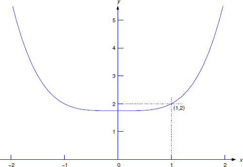
Find a solution of \[y'=x^3 \nonumber\] such that \(y(1)=2\).
Solution
At the beginning of this section we saw that the solutions of \(y'=x^3\) are
\[y={x^4\over4}+c. \nonumber\]
To determine a value of \(c\) such that \(y(1)=2\), we set \(x=1\) and \(y=2\) here to obtain
\[2=y(1)={1\over4}+c \nonumber\]
so
\[c={7\over4}. \nonumber\]
Therefore the required solution is
\[y={x^4+7\over4}. \nonumber\]
Figure 1.2.2 shows the graph of this solution. Note that imposing the condition \(y(1)=2\) is equivalent to requiring the graph of \(y\) to pass through the point \((1,2)\).
We can rewrite the problem considered in Example 1.2.5 more briefly as
\[y'=x^3,\quad y(1)=2.\nonumber\]
We call this an initial value problem. The requirement \(y(1)=2\) is an initial condition. Initial value problems can also be posed for higher order differential equations. For example,
\[\label{eq:1.2.11} y'' - 2y'+3y=e^x, \quad y(0)=1, \quad y'(0)=2\]
is an initial value problem for a second order differential equation where \(y\) and \(y'\) are required to have specified values at \(x=0\). In general, an initial value problem for an \(n\)-th order differential equation requires \(y\) and its first \(n-1\) derivatives to have specified values at some point \(x_0\). These requirements are the initial conditions.We’ll denote an initial value problem for a differential equation by writing the initial conditions after the equation, as in Equation \ref{eq:1.2.11}. For example, we would write an initial value problem for Equation \ref{eq:1.2.2} as
\[\label{eq:1.2.12} y^{(n)}=f(x,y,y', \dots,y^{(n-1)}),\, y(x_0)=k_0,\, y'(x_0)=k_1,\, \dots,\, y^{(n-1)}=k_{n-1}.\]
Consistent with our earlier definition of a solution of the differential equation in Equation \ref{eq:1.2.12}, we say that \(y\) is a solution of the initial value problem Equation \ref{eq:1.2.12} if \(y\) is \(n\) times differentiable and
\[y^{(n)}(x)=f(x,y(x),y'(x), \dots,y^{(n-1)}(x))\nonumber\]
for all \(x\) in some open interval \((a,b)\) that contains \(x_0\), and \(y\) satisfies the initial conditions in Equation \ref{eq:1.2.12}. The largest open interval that contains \(x_0\) on which \(y\) is defined and satisfies the differential equation is the interval of validity of \(y\).
In Example 1.2.5 we saw that
\[\label{eq:1.2.13} y={x^4+7\over4}\]
is a solution of the initial value problem
\[y'=x^3,\quad y(1)=2.\nonumber\]
Since the function in Equation \ref{eq:1.2.13} is defined for all \(x\), the interval of validity of this solution is \((-\infty,\infty)\).
In Example 1.2.2 we verified that
\[\label{eq:1.2.14} y={x^2\over3}+{1\over x}\]
is a solution of
\[xy'+y=x^2 \nonumber\]
on \((0,\infty)\) and on \((-\infty,0)\). By evaluating Equation \ref{eq:1.2.14} at \(x=\pm1\), you can see that Equation \ref{eq:1.2.14} is a solution of the initial value problems
\[\label{eq:1.2.15} xy'+y=x^2,\quad y(1)={4\over3}\]
and
\[\label{eq:1.2.16} xy'+y=x^2,\quad y(-1)=-{2\over3}.\]
The interval of validity of Equation \ref{eq:1.2.14} as a solution of Equation \ref{eq:1.2.15} is \((0,\infty)\), since this is the largest interval that contains \(x_0=1\) on which Equation \ref{eq:1.2.14} is defined. Similarly, the interval of validity of Equation \ref{eq:1.2.14} as a solution of Equation \ref{eq:1.2.16} is \((-\infty,0)\), since this is the largest interval that contains \(x_0=-1\) on which Equation \ref{eq:1.2.14} is defined.
Free Fall Under Constant Gravity
The term initial value problem originated in problems of motion where the independent variable is \(t\) (representing elapsed time), and the initial conditions are the position and velocity of an object at the initial (starting) time of an experiment.
An object falls under the influence of gravity near Earth’s surface, where it can be assumed that the magnitude of the acceleration due to gravity is a constant \(g\).
- Construct a mathematical model for the motion of the object in the form of an initial value problem for a second order differential equation, assuming that the altitude and velocity of the object at time \(t=0\) are known. Assume that gravity is the only force acting on the object.
- Solve the initial value problem derived above to obtain the altitude as a function of time.
Solution a
Let \(y(t)\) be the altitude of the object at time \(t\). Since the acceleration of the object has constant magnitude \(g\) and is in the downward (negative) direction, \(y\) satisfies the second order equation
\[y''=-g, \nonumber\]
where the prime now indicates differentiation with respect to \(t\). If \(y_0\) and \(v_0\) denote the altitude and velocity when \(t=0\), then \(y\) is a solution of the initial value problem
\[\label{eq:1.2.17} y''=-g,\quad y(0)=y_0,\quad y'(0)=v_0.\]
Solution b
Integrating Equation \ref{eq:1.2.17} twice yields
\[\begin{aligned} y'&=-gt+c_1, \\ y&=-{gt^2\over2}+c_1t+c_2.\end{aligned}\]
Imposing the initial conditions \(y(0)=y_0\) and \(y'(0)=v_0\) in these two equations shows that \(c_1=v_0\) and \(c_2=y_0\). Therefore the solution of the initial value problem Equation \ref{eq:1.2.17} is
\[y=- {gt^2\over2}+v_0t+y_0. \nonumber\]