6.1: Spring Problems I

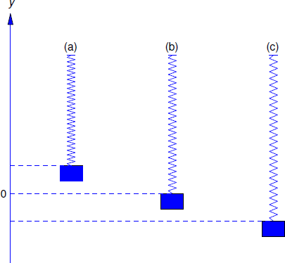
We consider the motion of an object of mass \(m\), suspended from a spring of negligible mass. We say that the spring–mass system is in equilibrium when the object is at rest and the forces acting on it sum to zero. The position of the object in this case is the equilibrium position. We define \(y\) to be the displacement of the object from its equilibrium position (Figure 6.1.1 ), measured positive upward.

Figure 6.1.1 : (a) \(y > 0\) (b) \(y = 0\), (c) \(y < 0\)

Our model accounts for the following kinds of forces acting on the object:

• The force \(-mg\), due to gravity.
• A force \(F_s\) exerted by the spring resisting change in its length. The natural length of the spring is its length with no mass attached. We assume that the spring obeys Hooke’s law: If the length of the spring is changed by an amount \(\Delta L\) from its natural length, then the spring exerts a force \(F_s=k\Delta L\), where \(k\) is a positive number called the spring constant. If the spring is stretched then \(\Delta L>0\) and \(F_s>0\), so the spring force is upward, while if the spring is compressed then \(\Delta L<0\) and \(F_s<0\), so the spring force is downward.
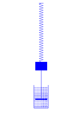
• A damping force \(F_d=-cy'\) that resists the motion with a force proportional to the velocity of the object. It may be due to air resistance or friction in the spring. However, a convenient way to visualize a damping force is to assume that the object is rigidly attached to a piston with negligible mass immersed in a cylinder (called a dashpot) filled with a viscous liquid (Figure 6.1.1 ). As the piston moves, the liquid exerts a damping force. We say that the motion is undamped if \(c=0\), or damped if \(c>0\).
• An external force \(F\), other than the force due to gravity, that may vary with \(t\), but is independent of displacement and velocity. We say that the motion is free if \(F\equiv0\), or forced if \(F\not\equiv0\).

Figure 6.1.2 : A spring – mass system with damping

From Newton’s second law of motion,

\[\label{eq:6.1.1} my''=-mg+F_d+F_s+F=-mg-cy'+F_s+F.\]

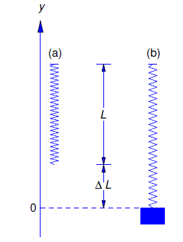
We must now relate \(F_s\) to \(y\). In the absence of external forces the object stretches the spring by an amount \(\Delta l\) to assume its equilibrium position (Figure 6.1.3 ). Since the sum of the forces acting on the object is then zero, Hooke’s Law implies that \(mg=k\Delta l\). If the object is displaced \(y\) units from its equilibrium position, the total change in the length of the spring is \(\Delta L=\Delta l-y\), so Hooke’s law implies that

\[F_s=k\Delta L=k\Delta l-ky.\nonumber \]

Substituting this into Equation \ref{eq:6.1.1} yields

\[my''=-mg-cy'+k\Delta L-ky+F.\nonumber \]

Since \(mg=k\Delta l\) this can be written as

\[\label{eq:6.1.2} my''+cy'+ky=F.\]

We call this the equation of motion.

Figure 6.1.3 :(a) Natural length of spring   (b) Spring stretched by mass

Simple Harmonic Motion

Throughout the rest of this section we’ll consider spring–mass systems without damping; that is, \(c=0\). We’ll consider systems with damping in the next section. We first consider the case where the motion is also free; that is, \(F\)=0. We begin with an example.

Example 6.1.1

An object stretches a spring \(6\) inches in equilibrium.

1. Set up the equation of motion and find its general solution.
2. Find the displacement of the object for \(t>0\) if it is initially displaced 18 inches above equilibrium and given a downward velocity of \(3\) ft/s.

Solution a:

Setting \(c=0\) and \(F=0\) in Equation \ref{eq:6.1.2} yields the equation of motion

\[my''+ky=0,\nonumber \]

which we rewrite as

\[\label{eq:6.1.3} y''+{k\over m}y=0.\]

Although we would need the weight of the object to obtain \(k\) from the equation \(mg=k\Delta l\) we can obtain \(k/m\) from \(\Delta l\) alone; thus, \(k/m=g/\Delta l\). Consistent with the units used in the problem statement, we take \(g=32\) ft/s\(^2\). Although \(\Delta l\) is stated in inches, we must convert it to feet to be consistent with this choice of \(g\); that is, \(\Delta l =1/2\) ft. Therefore

\[{k\over m}={32\over1/2}=64\nonumber \]

and Equation \ref{eq:6.1.3} becomes

\[\label{eq:6.1.4} y''+64y=0.\]

The characteristic equation of Equation \ref{eq:6.1.4} is

\[r^2+64=0,\nonumber \]

which has the zeros \(r=\pm 8i\). Therefore the general solution of Equation \ref{eq:6.1.4} is

\[\label{eq:6.1.5} y=c_1\cos8t+c_2\sin8t.\]

Solution b:

The initial upward displacement of 18 inches is positive and must be expressed in feet. The initial downward velocity is negative; thus,

\[y(0)={3\over2}\quad \text{and} \quad y'(0)=-3.\nonumber \]

Differentiating Equation \ref{eq:6.1.5} yields

\[\label{eq:6.1.6} y'=-8c_1\sin8t+8c_2\cos8t.\]

Setting \(t=0\) in Equation \ref{eq:6.1.5} and Equation \ref{eq:6.1.6} and imposing the initial conditions shows that \(c_1=3/2\) and \(c_2=-3/8\). Therefore

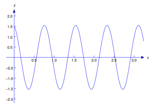
\[y={3\over2}\cos8t-{3\over8}\sin8t,\nonumber \]

where \(y\) is in feet (Figure 6.1.4 ).

We’ll now consider the equation

\[my''+ky=\nonumber 0\]

where \(m\) and \(k\) are arbitrary positive numbers. Dividing through by \(m\) and defining \(\omega_0=\sqrt{k/m}\) yields

\[y''+\omega_0^2y=0.\nonumber \]

The general solution of this equation is

\[\label{eq:6.1.7} y=c_1\cos\omega_0t+c_2\sin\omega_0t.\]

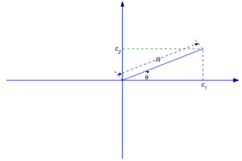
We can rewrite this in a more useful form by defining

\[\label{eq:6.1.8} R=\sqrt{c_1^2+c_2^2},\]

Figure 6.1.4 : \(y=\frac{3}{2}\cos 8t -\frac{3}{8}\sin 8t\)

and

\[\label{eq:6.1.9} c_1=R\cos\phi\quad \text{and} \quad c_2=R\sin\phi.\]

Substituting from Equation \ref{eq:6.1.9} into Equation \ref{eq:6.1.7} and applying the identity

\[\cos\omega_0t\cos\phi+\sin\omega_0t\sin\phi=\cos(\omega_0t-\phi)\nonumber \]

yields

\[\label{eq:6.1.10} y=R\cos(\omega_0t-\phi).\]

From Equation \ref{eq:6.1.8} and Equation \ref{eq:6.1.9} we see that the \(R\) and \(\phi\) can be interpreted as polar coordinates of the point with rectangular coordinates \((c_1,c_2)\) (Figure 6.1.5 ). Given \(c_1\) and \(c_2\), we can compute \(R\) from Equation \ref{eq:6.1.8}. From Equation \ref{eq:6.1.8} and Equation \ref{eq:6.1.9}, we see that \(\phi\) is related to \(c_1\) and \(c_2\) by

\[\cos\phi={c_1\over\sqrt{c_1^2+c_2^2}}\quad \text{and} \quad\sin\phi= {c_2\over\sqrt{c_1^2+c_2^2}}.\nonumber \]

There are infinitely many angles \(\phi\), differing by integer multiples of \(2\pi\), that satisfy these equations. We will always choose \(\phi\) so that \(-\pi\le\phi<\pi\).

The motion described by Equation \ref{eq:6.1.7} or Equation \ref{eq:6.1.10} is simple harmonic motion. We see from either of these equations that the motion is periodic, with period

\[T=2\pi/\omega_0.\nonumber \]

This is the time required for the object to complete one full cycle of oscillation (for example, to move from its highest position to its lowest position and back to its highest position). Since the highest and lowest positions of the object are \(y=R\) and \(y=-R\), we say that \(R\) is the amplitude of the oscillation. The angle \(\phi\) in Equation \ref{eq:6.1.10} is the phase angle. It’s measured in radians. Equation Equation \ref{eq:6.1.10} is the amplitude–phase form of the displacement. If \(t\) is in seconds then \(\omega_0\) is in radians per second (rad/s); it is the frequency of the motion. It is also called the natural frequency of the spring–mass system without damping.

Figure 6.1.5 : \(R=\sqrt{c_{1}^{2}+c_{2}^{2}}\); \(c_{1}=R\cos\phi\); \(c_{2}=R\sin\phi\)

Example 6.1.2

We found the displacement of the object in Example 6.1.1 to be

\[y={3\over2}\cos8t-{3\over8}\sin8t.\nonumber \]

Find the frequency, period, amplitude, and phase angle of the motion.

Solution:

The frequency is \(\omega_0=8\) rad/s, and the period is \(T=2\pi/\omega_0=\pi/4\) s. Since \(c_1=3/2\) and \(c_2=-3/8\), the amplitude is

\[R=\sqrt{c^2_1+c^2_2}=\sqrt{\left({3\over2}\right)^2+\left({3\over8}\right)^2} ={3\over8}\sqrt{17}.\nonumber \]

The phase angle is determined by

\[\label{eq:6.1.11} \cos\phi = \frac{\frac{3}{2}}{\frac{3}{8}\sqrt{17}} = \frac{4}{\sqrt{17}}\]

and

\[\label{eq:6.1.12} \sin\phi={-{3\over8}\over{3\over8}\sqrt{17}}=-{1\over\sqrt{17}}.\]

Using a calculator, we see from Equation \ref{eq:6.1.11} that

\[\phi\approx\pm.245\mbox{ rad}.\nonumber \]

Since \(\sin\phi<0\) (see Equation \ref{eq:6.1.12}), the minus sign applies here; that is,

\[\phi\approx-.245\mbox{ rad}.\nonumber \]

Example 6.1.3

The natural length of a spring is 1 m. An object is attached to it and the length of the spring increases to 102 cm when the object is in equilibrium. Then the object is initially displaced downward 1 cm and given an upward velocity of 14 cm/s. Find the displacement for \(t>0\). Also, find the natural frequency, period, amplitude, and phase angle of the resulting motion. Express the answers in cgs units.

Solution:

In cgs units \(g=980\) cm/s\(^2\). Since \(\Delta l=2\) cm, \(\omega_0^2=g/\Delta l=490\). Therefore

\[y''+490y=0, \quad y(0)=-1,\quad y'(0)=14.\nonumber \]

The general solution of the differential equation is

\[y=c_1\cos7\sqrt{10}t+c_2\sin7\sqrt{10}t,\nonumber \]

so

\[y'=7\sqrt{10}\left(-c_1\sin7\sqrt{10}t+c_2\cos7\sqrt{10}t\right).\nonumber \]

Substituting the initial conditions into the last two equations yields \(c_1=-1\) and \(c_2=2/\sqrt{10}\). Hence,

\[y=-\cos7\sqrt{10}t+{2\over\sqrt{10}}\sin7\sqrt{10}t.\nonumber \]

The frequency is \(7\sqrt{10}\) rad/s, and the period is \(T=2\pi/(7\sqrt{10})\) s. The amplitude is

\[R=\sqrt{c_{1}^{2}+c_{2}^{2}}=\sqrt{(-1)^{2}+\left(\frac{2}{\sqrt{10}} \right)^{2}}=\sqrt{\frac{7}{5}}\text{cm}\nonumber \]

The phase angle is determined by

\[\cos\phi = \frac{c_{1}}{R}=-\sqrt{\frac{5}{7}}\quad\text{and}\quad\sin\phi = \frac{c_{2}}{R}=\sqrt{\frac{2}{7}}\nonumber \]

Therefore \(\phi\) is in the second quadrant and

\[\phi = \cos ^{-1}\left(-\sqrt{\frac{5}{7}} \right)\approx 2.58\text{rad}\nonumber \]

Undamped Forced Oscillation

In many mechanical problems a device is subjected to periodic external forces. For example, soldiers marching in cadence on a bridge cause periodic disturbances in the bridge, and the engines of a propeller driven aircraft cause periodic disturbances in its wings. In the absence of sufficient damping forces, such disturbances – even if small in magnitude – can cause structural breakdown if they are at certain critical frequencies. To illustrate, this we’ll consider the motion of an object in a spring–mass system without damping, subject to an external force

\[F(t)=F_0\cos\omega t\nonumber \]

where \(F_0\) is a constant. In this case the equation of motion Equation \ref{eq:6.1.2} is

\[my''+ky=F_0\cos\omega t,\nonumber \]

which we rewrite as

\[\label{eq:6.1.13} y''+\omega_0^2y={F_0\over m}\cos\omega t\]

with \(\omega_0=\sqrt{k/m}\). We’ll see from the next two examples that the solutions of Equation \ref{eq:6.1.13} with \(\omega\ne\omega_0\) behave very differently from the solutions with \(\omega=\omega_0\).

Example 6.1.4

Solve the initial value problem

\[\label{eq:6.1.14} y''+\omega_0^2y={F_0\over m}\cos\omega t, \quad y(0)=0,\quad y'(0)=0,\]

given that \(\omega\ne\omega_0\).

Solution:

We first obtain a particular solution of Equation \ref{eq:6.1.13} by the method of undetermined coefficients. Since \(\omega\ne\omega _0\), \(\cos\omega t\) isn’t a solution of the complementary equation

\[y''+\omega_0^2y=0.\nonumber \]

Therefore Equation \ref{eq:6.1.13} has a particular solution of the form

\[y_p=A\cos\omega t+B\sin\omega t.\nonumber \]

Since

\[y''_p=-\omega^2(A\cos\omega t+B\sin\omega t),\nonumber \]

\[y_p''+\omega_0^2y_p={F_0\over m}\cos\omega t\nonumber \]

if and only if

\[(\omega_0^2-\omega^2)\left(A\cos\omega t+ B\sin\omega t\right)={F_0\over m}\cos\omega t.\nonumber \]

This holds if and only if

\[A={F_0\over m(\omega_0^2-\omega^2)}\quad \text{and} \quad B=0,\nonumber \]

so

\[y_p={F_0\over m(\omega_0^2-\omega^2)}\cos\omega t.\nonumber \]

The general solution of Equation \ref{eq:6.1.13} is

\[\label{eq:6.1.15} y={F_0\over m(\omega_0^2-\omega^2)}\cos\omega t +c_1\cos\omega_0 t+c_2\sin\omega_0t,\]

so

\[y'={-\omega F_0\over m(\omega_0^2-\omega^2)}\sin\omega t +\omega_0(-c_1\sin\omega_0 t+c_2\cos\omega_0t).\nonumber \]

The initial conditions \(y(0)=0\) and \(y'(0)=0\) in Equation \ref{eq:6.1.14} imply that

\[c_1=-{F_0\over m(\omega_0^2-\omega^2)}\quad \text{and} \quad c_2=0.\nonumber \]

Substituting these into Equation \ref{eq:6.1.15} yields

\[\label{eq:6.1.16} y={F_0\over m(\omega_0^2-\omega^2)}(\cos\omega t-\cos\omega _0t).\]

It is revealing to write this in a different form. We start with the trigonometric identities

\[\begin{aligned} \cos(\alpha-\beta)&=\cos\alpha\cos\beta+\sin\alpha\sin\beta\\ \cos(\alpha+\beta)&=\cos\alpha\cos\beta-\sin\alpha\sin\beta.\end{aligned}\nonumber \]

Subtracting the second identity from the first yields

\[\label{eq:6.1.17} \cos(\alpha-\beta)-\cos(\alpha+\beta)=2\sin\alpha\sin\beta\]

Now let

\[\label{eq:6.1.18} \alpha-\beta=\omega t\quad \text{and} \quad\alpha+\beta=\omega_0t,\]

so that

\[\label{eq:6.1.19} \alpha={(\omega_0+\omega)t\over2}\quad \text{and} \quad \beta={(\omega_0-\omega)t\over2}.\]

Substituting Equation \ref{eq:6.1.18} and Equation \ref{eq:6.1.19} into Equation \ref{eq:6.1.17} yields

\[\cos\omega t-\cos\omega_0t= 2\sin{(\omega_0-\omega)t\over2}\sin{(\omega_0+\omega)t\over2},\nonumber \]

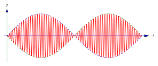
and substituting this into Equation \ref{eq:6.1.16} yields

\[\label{eq:6.1.20} y=R(t)\sin{(\omega_0+\omega)t\over2},\]

where

\[\label{eq:6.1.21} R(t)={2F_0\over m(\omega_0^2-\omega^2)} \sin{(\omega_0-\omega)t\over2}.\]

From Equation \ref{eq:6.1.20} we can regard \(y\) as a sinusoidal variation with frequency \((\omega_0+\omega)/2\) and variable amplitude \(|R(t)|\). In Figure 6.1.6 the dashed curve above the \(t\) axis is \(y=|R(t)|\), the dashed curve below the \(t\) axis is \(y=-|R(t)|\), and the displacement \(y\) appears as an oscillation bounded by them. The oscillation of \(y\) for \(t\) on an interval between successive zeros of \(R(t)\) is called a beat.

Figure 6.1.6 : Undamped oscillation with beats

You can see from Equation \ref{eq:6.1.20} and Equation \ref{eq:6.1.21} that

\[|y(t)|\le{2|F_0|\over m|\omega_0^2-\omega^2|};\nonumber \]

moreover, if \(\omega+\omega_0\) is sufficiently large compared with \(\omega -\omega_0\), then \(|y|\) assumes values close to (perhaps equal to) this upper bound during each beat. However, the oscillation remains bounded for all \(t\). (This assumes that the spring can withstand deflections of this size and continue to obey Hooke’s law.) The next example shows that this isn’t so if \(\omega=\omega_0\).

Example 6.1.5

Find the general solution of

\[\label{eq:6.1.22} y''+\omega_0^2y={F_0\over m}\cos\omega_0t.\]

Solution:

We first obtain a particular solution \(y_p\) of Equation \ref{eq:6.1.22}. Since \(\cos\omega_0t\) is a solution of the complementary equation, the form for \(y_p\) is

\[\label{eq:6.1.23} y_p=t(A\cos\omega_0t+B\sin\omega_0t).\]

Then

\[y_p'=A\cos\omega_0t+B\sin\omega_0t +\omega_0t(-A\sin\omega_0t+B\cos\omega_0t)\nonumber \]

and

\[\label{eq:6.1.24} y''_p=2\omega_0(-A\sin\omega_0t +B\cos\omega_0t)-\omega_0^2t(A\cos\omega_0t+B\sin\omega_0t).\]

From Equation \ref{eq:6.1.23} and Equation \ref{eq:6.1.24}, we see that \(y_p\) satisfies Equation \ref{eq:6.1.22} if

\[-2A\omega_0\sin\omega_0t+2B\omega_0\cos\omega_0t={F_0\over m} \cos\omega_0t;\nonumber \]

that is, if

\[A=0\quad \text{and} \quad B={F_0\over2m\omega_0}.\nonumber \]

Therefore

\[y_p={F_0t\over2m\omega_0}\sin\omega_0t\nonumber \]

is a particular solution of Equation \ref{eq:6.1.22}. The general solution of Equation \ref{eq:6.1.22} is

\[y={F_0t\over2m\omega_0}\sin\omega_0t+c_1\cos\omega_0t+c_2\sin\omega_0t.\nonumber \]

Figure 6.1.7 : Undamped displacement due to resonance.

The graph of \(y_p\) is shown in Figure 6.1.7 , where it can be seen that \(y_p\) oscillates between the dashed lines

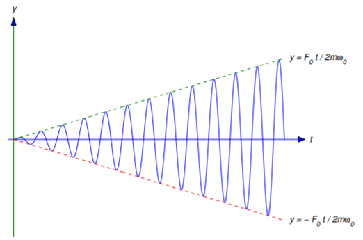
\[y={F_0t\over2m\omega_0}\quad \text{and} \quad y=-{F_0t\over2m\omega_0}\nonumber \]

with increasing amplitude that approaches \(\infty\) as \(t\to\infty\). Of course, this means that the spring must eventually fail to obey Hooke’s law or break.

This phenomenon of unbounded displacements of a spring–mass system in response to a periodic forcing function at its natural frequency is called resonance. More complicated mechanical structures can also exhibit resonance–like phenomena. For example, rhythmic oscillations of a suspension bridge by wind forces or of an airplane wing by periodic vibrations of reciprocating engines can cause damage or even failure if the frequencies of the disturbances are close to critical frequencies determined by the parameters of the mechanical system in question.