
12.1: The Heat Equation
- Page ID
- 9467

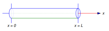
We begin the study of partial differential equations with the problem of heat flow in a uniform bar of length \(L\), situated on the \(x\) axis with one end at the origin and the other at \(x = L\) (Figure 12.1.1 ).
We assume that the bar is perfectly insulated except possibly at its endpoints, and that the temperature is constant on each cross section and therefore depends only on \(x\) and \(t\). We also assume that the thermal properties of the bar are independent of \(x\) and \(t\). In this case, it can be shown that the temperature \(u = u(x, t)\) at time \(t\) at a point \(x\) units from the origin satisfies the partial differential equation
\[u_{t}=a^{2}u_{xx},\quad 0<x<L,\quad t>0,\nonumber\]
where \(a\) is a positive constant determined by the thermal properties. This is the heat equation.
To determine \(u\), we must specify the temperature at every point in the bar when \(t=0\), say
\[u(x,0)=f(x),\quad 0\le x\le L. \nonumber \]
We call this the initial condition. We must also specify boundary conditions that \(u\) must satisfy at the ends of the bar for all \(t>0\). We’ll call this problem an initial-boundary value problem.
We begin with the boundary conditions \(u(0,t)=u(L,t)=0\), and write the initial-boundary value problem as
\[\label{eq:12.1.1} \begin{array}{c}{u_{t}=a^{2}u_{xx},\quad 0<x<L,\quad t>0,}\\{u(0,t)=0,\quad u(L,t)=0,\quad t>0,}\\{u(x,0)=f(x),\quad 0\leq x\leq L.}\end{array}\]
Our method of solving this problem is called separation of variables (not to be confused with method of separation of variables used in Section 2.2 for solving ordinary differential equations). We begin by looking for functions of the form
\[v(x,t)=X(x)T(t) \nonumber \]
that are not identically zero and satisfy
\[v_t=a^2v_{xx},\quad v(0,t)=0,\quad v(L,t)=0 \nonumber \]
for all \((x,t)\). Since
\[v_t=XT' \quad \text{and} \quad v_{xx}=X''T, \nonumber \]
\(v_t=a^2v_{xx}\) if and only if
\[XT'=a^2X''T, \nonumber \]
which we rewrite as
\[{T'\over a^2T}={X''\over X}. \nonumber \]
Since the expression on the left is independent of \(x\) while the one on the right is independent of \(t\), this equation can hold for all \((x,t)\) only if the two sides equal the same constant, which we call a separation constant, and write it as \(-\lambda\); thus,
\[{X''\over X}={T'\over a^2T}=-\lambda. \nonumber \]
This is equivalent to
\[X''+\lambda X=0 \nonumber \]
and
\[\label{eq:12.1.2} T'=-a^2\lambda T.\]
Since \(v(0,t)=X(0)T(t)=0\) and \(v(L,t)=X(L)T(t)=0\) and we don’t want \(T\) to be identically zero, \(X(0)=0\) and \(X(L)=0\). Therefore \(\lambda\) must be an eigenvalue of the boundary value problem
\[\label{eq:12.1.3} X''+\lambda X=0,\quad X(0)=0,\quad X(L)=0,\]
and \(X\) must be a \(\lambda\)-eigenfunction. From Theorem 11.1.2, the eigenvalues of Equation \ref{eq:12.1.3} are \(\lambda_n=n^2\pi^2/L^2\), with associated eigenfunctions
\[X_n=\sin{n\pi x\over L}, \quad n=1,2,3,\dots. \nonumber \]
Substituting \(\lambda=n^2\pi^2/L^2\) into Equation \ref{eq:12.1.2} yields
\[T'=-(n^2\pi^2a^2/L^2)T, \nonumber \]
which has the solution
\[T_n=e^{-n^2\pi^2a^2t/L^2}. \nonumber \]
Now let
\[v_n(x,t)=X_n(x)T_n(t)=e^{-n^2\pi^2a^2t/L^2}\sin{n\pi x\over L},\quad n=1,2,3,\dots \nonumber \]
Since
\[v_n(x,0)=\sin{n\pi x\over L}, \nonumber \]
\(v_n\) satisfies Equation \ref{eq:12.1.1} with \(f(x)=\sin n\pi x/L\). More generally, if \(\alpha_1,\dots,\alpha_m\) are constants and
\[u_m(x,t)= \sum_{n=1}^m \alpha_ne^{-n^2\pi^2a^2t/L^2}\sin{n\pi x\over L}, \nonumber \]
then \(u_m\) satisfies Equation \ref{eq:12.1.1} with
\[f(x)=\sum_{n=1}^m \alpha_n\sin{n\pi x\over L}. \nonumber \]
This motivates the next definition.
The formal solution of the initial-boundary value problem
\[\label{eq:12.1.4} \begin{array}{c}{u_{t}=a^{2}u_{xx},\quad 0<x<L,\quad t>0,}\\{u(0,t)=0,\quad u(L,t)=0,\quad t>0,}\\{u(x,0)=f(x),\quad 0\leq x\leq L}\end{array}\]
is
\[\label{eq:12.1.5} u(x,t)=\sum_{n=1}^\infty \alpha_ne^{-n^2\pi^2a^2t/L^2}\sin{n\pi x\over L},\]
where
\[S(x)=\sum_{n=1}^\infty \alpha_n\sin{n\pi x\over L} \nonumber \]
is the Fourier sine series of \(f\) on \([0,L]\); that is,
\[\alpha_n= \dfrac{2}{L} \int_0^L f(x) \sin \dfrac{n\pi x}{L} \,dx. \nonumber \]
We use the term “formal solution” in this definition because it is not in general true that the infinite series in Equation \ref{eq:12.1.5} actually satisfies all the requirements of the initial-boundary value problem Equation \ref{eq:12.1.4} when it does, we say that it is an actual solution of Equation \ref{eq:12.1.4}.
Because of the negative exponentials in Equation \ref{eq:12.1.5}, \(u\) converges for all \((x,t)\) with \(t>0\) (Exercise 12.1.54). Since each term in Equation \ref{eq:12.1.5} satisfies the heat equation and the boundary conditions in Equation \ref{eq:12.1.4}, \(u\) also has these properties if \(u_t\) and \(u_{xx}\) can be obtained by differentiating the series in Equation \ref{eq:12.1.5} term by term once with respect to \(t\) and twice with respect to \(x\), for \(t>0\). However, it is not always legitimate to differentiate an infinite series term by term. The next theorem gives a useful sufficient condition for legitimacy of term by term differentiation of an infinite series. We omit the proof.
A convergent infinite series
\[W(z)=\sum_{n=1}^\infty w_n(z) \nonumber\]
can be differentiated term by term on a closed interval \([z_1,z_2]\) to obtain
\[W'(z)=\sum_{n=1}^\infty w_n'(z) \nonumber\]
\((\)where the derivatives at \(z=z_1\) and \(z=z_2\) are one-sided\()\) provided that \(w_n'\) is continuous on \([z_1,z_2]\) and
\[|w_n'(z)|\le M_n,\quad z_1\le z\le z_2,\quad n=1,2,3,\dots, \nonumber\]
where \(M_1,\) \(M_2,\) …, \(M_n,\) …, are constants such that the series \(\sum_{n=1}^\infty M_n\) converges.
Theorem 12.1.2 , applied twice with \(z=x\) and once with \(z=t\), shows that \(u_{xx}\) and \(u_t\) can be obtained by differentiating \(u\) term by term if \(t>0\) (Exercise 12.1.54). Therefore \(u\) satisfies the heat equation and the boundary conditions in Equation \ref{eq:12.1.4} for \(t>0\). Therefore, since \(u(x,0)=S(x)\) for \(0\le x\le L\), \(u\) is an actual solution of Equation \ref{eq:12.1.4} if and only if \(S(x)=f(x)\) for \(0\le x\le L\). From Theorem 11.3.2, this is true if \(f\) is continuous and piecewise smooth on \([0,L]\), and \(f(0)=f(L)=0\).
In this chapter we’ll define formal solutions of several kinds of problems. When we ask you to solve such problems, we always mean that you should find a formal solution.
Solve Equation \ref{eq:12.1.4} with \(f(x)=x(x^2-3Lx+2L^2)\).
Solution
From Example [example:11.3.6}, the Fourier sine series of \(f\) on \([0,L]\) is
\[S(x)=\frac{12L^{3}}{\pi ^{3}}\sum_{n=1}^{\infty}\frac{1}{n^{3}}\sin \frac{n\pi x}{L}\nonumber\]
Therefore
\[u(x,t)=\frac{12L^{3}}{\pi ^{3}}\sum_{n=1}^{\infty }\frac{1}{n^{3}} e^{-n^{2}\pi ^{2}a^{2}t/L^{2}}\sin\frac{n\pi x}{L}\nonumber \]
If both ends of bar are insulated so that no heat can pass through them, then the boundary conditions are
\[u_x(0,t)=0,\quad u_x(L,t)=0,\quad t>0. \nonumber\]
We leave it to you (Exercise 12.1.1) to use the method of separation of variables and Theorem 11.1.3 to motivate the next definition.
The formal solution of the initial-boundary value problem
\[\label{eq:12.1.6} \begin{array}{c}{u_{t}=a^{2}u_{xx},\quad 0<x<L,\quad t>0,}\\{u_{x}(0,t)=0,\quad u_{x}(L,t)=0,\quad t>0,}\\{u(x,0)=f(x),\quad 0\leq x\leq L}\end{array}\]
is
\[u(x,t)=\alpha_0+\sum_{n=1}^\infty \alpha_ne^{-n^2\pi^2 a^2t/L^2}\cos{n\pi x\over L}, \nonumber\]
where
\[C(x)=\alpha_0+\sum_{n=1}^\infty \alpha_n\cos{n\pi x\over L} \nonumber\]
is the Fourier cosine series of \(f\) on \([0,L];\) that is,
\[\alpha_0={1\over L}\int_0^Lf(x)\,dx \quad \text{and} \quad \alpha_n={2\over L}\int_0^Lf(x)\cos{n\pi x\over L}\,dx,\quad n=1,2,3,\dots. \nonumber\]
Solve Equation \ref{eq:12.1.6} with \(f(x)=x\).
Solution
From Example 11.3.1, the Fourier cosine series of \(f\) on \([0,L]\) is
\[C(x)=\frac{L}{2}-\frac{4L}{\pi ^{2}}\sum_{n=1}^{\infty}\frac{1}{(2n-1)^{2}}\cos \frac{(2n-1)\pi x}{L}\nonumber \]
Therefore
\[u(x,t)={L\over2}-{4L\over\pi^2}\sum_{n=1}^\infty {1\over(2n-1)^2} e^{-(2n-1)^2\pi^2a^2t/L^2}\cos{(2n-1)\pi x\over L}. \nonumber\]
We leave it to you (Exercise 12.1.2) to use the method of separation of variables and Theorem 11.1.4 to motivate the next definition.
The formal solution of the initial-boundary value problem
\[\label{eq:12.1.7} \begin{array}{c}{u_{t}=a^{2}u_{xx},\quad 0<x<L,\quad t>0,}\\{u(0,t)=0,\quad u_{x}(L,t)=0,\quad t>0,}\\{u(x,0)=f(x),\quad 0\leq x\leq L}\end{array}\]
is
\[u(x,t)=\sum_{n=1}^\infty \alpha_ne^{-(2n-1)^2\pi^2a^2t/4L^2}\sin{(2n-1)\pi x\over2L},\nonumber\]
where
\[S_M(x)=\sum_{n=1}^\infty \alpha_n\sin{(2n-1)\pi x\over2L}\nonumber\]
is the mixed Fourier sine series of \(f\) on \([0,L];\) that is,
\[\alpha_n={2\over L}\int_0^Lf(x)\sin{(2n-1)\pi x\over2L}\,dx.\nonumber\]
Solve Equation \ref{eq:12.1.7} with \(f(x)=x\).
Solution
From Example 11.3.4, the mixed Fourier sine series of \(f\) on \([0,L]\) is
\[S_M(x)=-{8L\over\pi^2}\sum_{n=1}^\infty{(-1)^n\over(2n-1)^2} \sin{(2n-1)\pi x\over2L}. \nonumber\]
Therefore
\[u(x,t)=-{8L\over\pi^2}\sum_{n=1}^\infty{(-1)^n\over(2n-1)^2} e^{-(2n-1)^2\pi^2a^2t/4L^2}\sin{(2n-1)\pi x\over2L}. \nonumber\]
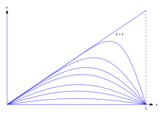
Figure 12.1.2 shows a graph of \(u=u(x,t)\) plotted with respect to \(x\) for various values of \(t\). The line \(y=x\) corresponds to \(t=0\). The other curves correspond to positive values of \(t\). As \(t\) increases, the graphs approach the line \(u=0\).
We leave it to you (Exercise 12.1.3) to use the method of separation of variables and Theorem 11.1.5 to motivate the next definition.
The formal solution of the initial-boundary value problem
\[\label{eq:12.1.8} \begin{array}{c}{u_{t}=a^{2}u_{xx},\quad 0<x<L,\quad t>0,}\\{u_{x}(0,t)=0,\quad u(L,t)=0,\quad t>0,}\\{u(x,0)=f(x),\quad 0\leq x\leq L}\end{array}\]
is
\[u(x,t)=\sum_{n=1}^\infty \alpha_ne^{-(2n-1)^2\pi^2a^2t/4L^2}\cos{(2n-1)\pi x\over2L},\nonumber\]
where
\[C_M(x)=\sum_{n=1}^\infty \alpha_n\cos{(2n-1)\pi x\over2L}\nonumber\]
is the mixed Fourier cosine series of \(f\) on \([0,L]\); that is,
\[\alpha_n={2\over L}\int_0^Lf(x)\cos{(2n-1)\pi x\over2L}\,dx.\nonumber\]
Solve Equation \ref{eq:12.1.8} with \(f(x)=x-L\).
Solution
From Example 11.3.3, the mixed Fourier cosine series of \(f\) on \([0,L]\) is
\[C_M(x)=-{8L\over\pi^2}\sum_{n=1}^\infty{1\over(2n-1)^2} \cos{(2n-1)\pi x\over2L}.\nonumber\]
Therefore
\[u(x,t)=-{8L\over\pi^2}\sum_{n=1}^\infty{1\over(2n-1)^2} e^{-(2n-1)^2\pi^2a^2t/4L^2}\cos{(2n-1)\pi x\over2L}.\nonumber\]
Nonhomogeneous Problems
A problem of the form
\[\label{eq:12.1.9} \begin{array}{c}{u_{t}=a^{2}u_{xx}+h(x),\quad 0<x<L,\quad t>0,}\\{u(0,t)=u_{0},\quad u(L,t)=u_{L},\quad t>0,}\\{u(x,0)=f(x),\quad 0\leq x\leq L}\end{array}\]
can be transformed to a problem that can be solved by separation of variables. We write
\[\label{eq:12.1.10} u(x,t)=v(x,t)+q(x),\]
where \(q\) is to be determined. Then
\[u_t=v_t \quad \text{and} \quad u_{xx}=v_{xx}+q''\nonumber\]
so \(u\) satisfies Equation \ref{eq:12.1.9} if \(v\) satisfies
\[\begin{array}{c}{v_{t}=a^{2}v_{xx}+a^{2}q''(x)+h(x),\quad 0<x<L,\quad t>0,}\\{v(0,t)=u_{0}-q(0),\quad v(L,t)=u_{L}-q(L),\quad t>0,}\\{v(x,0)=f(x)-q(x),\quad 0\leq x\leq L.}\end{array}\nonumber \]
This reduces to
\[\label{eq:12.1.11} \begin{array}{c}{v_{t}=a^{2}v_{xx},\quad 0<x<L,\quad t>0,}\\{v(0,t)=0,\quad v(L,t)=0,\quad t>0,}\\{v(x,0)=f(x)-q(x),\quad 0\leq x\leq L}\end{array}\]
if
\[a^2q''+h(x)=0,\quad q(0)=u_0,\quad q(L)=u_L.\nonumber\]
We can obtain \(q\) by integrating \(q''=-h/a^2\) twice and choosing the constants of integration so that \(q(0)=u_0\) and \(q(L)=u_L\). Then we can solve Equation \ref{eq:12.1.11} for \(v\) by separation of variables, and Equation \ref{eq:12.1.10} is the solution of Equation \ref{eq:12.1.9}.
Solve
\[\begin{array}{c}{u_{t}=u_{xx}-2,\quad 0<x<1,\quad t>0,}\\{u(0,t)=-1,\quad u(1,t)=1,\quad t>0,}\\{u(x,0)=x^{3}-2x^{2}+3x-1,\quad 0\leq x\leq 1.}\end{array}\nonumber \]
Solution
We leave it to you to show that
\[q(x)=x^2+x-1\nonumber\]
satisfies
\[q''-2=0,\quad q(0)=-1,\quad q(1)=1.\nonumber\]
Therefore
\[u(x,t)=v(x,t)+x^2+x-1,\nonumber\]
where
\[v_{t}=v_{xx},\quad 0<x<1,\quad t>0,\nonumber \]
\[v(0,t)=0,\quad v(1,t)=0,\quad t>0,\nonumber\]
and
\[v(x,0)=x^3-2x^2+3x-1-x^2-x+1=x(x^2-3x+2).\nonumber\]
From Example 12.1.1 with \(a=1\) and \(L=1\),
\[v(x,t)= {12\over\pi^3}\sum_{n=1}^\infty{1\over n^3} e^{-n^2\pi^2t}\sin n\pi x.\nonumber\]
Therefore
\[u(x,t)=x^2+x-1+ {12\over\pi^3}\sum_{n=1}^\infty{1\over n^3} e^{-n^2\pi^2t}\sin n\pi x. \nonumber\]
A similar procedure works if the boundary conditions in Equation \ref{eq:12.1.11} are replaced by mixed boundary conditions
\[u_x(0,t)=u_0,\quad u(L,t)=u_L,\quad t>0\nonumber\]
or
\[u(0,t)=u_0,\quad u_x(L,t)=u_L,\quad t>0;\nonumber\]
however, this isn’t true in general for the boundary conditions
\[u_x(0,t)=u_0,\quad u_x(L,t)=u_L,\quad t>0.\nonumber\]
(See Exercise 12.1.47.)
Using Technology
Numerical experiments can enhance your understanding of the solutions of initial-boundary value problems. To be specific, consider the formal solution
\[u(x,t)=\sum_{n=1}^\infty \alpha_ne^{-n^2\pi^2a^2t/L^2}\sin{n\pi x\over L},\nonumber\]
of Equation \ref{eq:12.1.4}, where
\[S(x)=\sum_{n=1}^\infty \alpha_n \sin{n\pi x \over L}\nonumber\]
is the Fourier sine series of \(f\) on \([0,L]\). Consider the \(m\)-th partial sum
\[\label{eq:12.1.12} u_m(x,t)=\sum_{n=1}^m \alpha_ne^{-n^2\pi^2a^2t/L^2}\sin{n\pi x\over L}.\]
For several fixed values of \(t\) (including \(t=0\)), graph \(u_m(x,t)\) versus \(t\). In some cases it may be useful to graph the curves corresponding to the various values of \(t\) on the same axes in other cases you may want to graph the various curves successively (for increasing values of \(t\)), and create a primitive motion picture on your monitor. Repeat this experiment for several values of \(m\), to compare how the results depend upon \(m\) for small and large values of \(t\). However, keep in mind that the meanings of “small” and “large” in this case depend upon the constants \(a^2\) and \(L^2\). A good way to handle this is to rewrite Equation \ref{eq:12.1.12} as
\[u_m(x,t)=\sum_{n=1}^m \alpha_ne^{-n^2\tau}\sin{n\pi x\over L},\nonumber\]
where
\[\label{eq:12.1.13} \tau={\pi^2a^2t\over L^2},\]
and graph \(u_m\) versus \(x\) for selected values of \(\tau\).
These comments also apply to the situations considered in Definitions 12.1.3 -12.1.5 , except that Equation \ref{eq:12.1.13} should be replaced by
\[\tau={\pi^2a^2t\over 4L^2},\nonumber\]
in Definitions 12.1.4 and 12.1.5 .