1.4: Applications
- Page ID
- 90911

Conservation Laws
There are many applications of quasilinear equations, especially in fluid dynamics. The advection equation is one such example and generalizations of this example to nonlinear equations leads to some interesting problems. These equations fall into a category of equations called conservation laws. We will first discuss one-dimensional (in space) conservations laws and then look at simple examples of nonlinear conservation laws.
Conservation laws are useful in modeling several systems. They can be boiled down to determining the rate of change of some stuff, \(Q(t)\), in a region, \(a ≤ x ≤ b\), as depicted in Figure \(\PageIndex{1}\). The simples model is to think of fluid flowing in one dimension, such as water flowing in a stream. Or, it could be the transport of mass, such as a pollutant. One could think of traffic flow down a straight road.
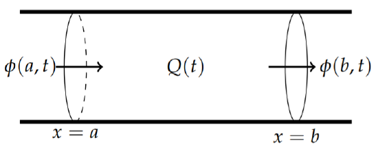
This is an example of a typical mixing problem. The rate of change of \(Q(t)\) is given as
\[\text{the rate of change of }Q=\text{ Rate in }-\text{ Rate Out }+\text{ source term.}\nonumber\]
Here the “Rate in” is how much is flowing into the region in Figure \(\PageIndex{1}\) from the \(x = a\) boundary. Similarly, the “Rate out” is how much is flowing into the region from the \(x = b\) boundary. [Of course, this could be the other way, but we can imagine for now that \(q\) is flowing from left to right.] We can describe this flow in terms of the flux, \(\phi (x, t)\) over the ends of the region. On the left side we have a gain of \(\phi (a, t)\) and on the right side of the region there is a loss of \(\phi (b, t)\).
The source term would be some other means of adding or removing \(Q\) from the region. In terms of fluid flow, there could be a source of fluid inside the region such as a faucet adding more water. Or, there could be a drain letting water escape. We can denote this by the total source over the interval, \(\int_a^b f(x, t)\: dx\). Here \(f(x, t)\) is the source density.
In summary, the rate of change of \(Q(x, t)\) can be written as
\[\frac{dQ}{dt}=\phi (a,t)-\phi (b,t)+\int_a^b f(x,y)dx.\nonumber\]
We can write this in a slightly different form by noting that \(\phi (a, t) −\phi (b, t)\) can be viewed as the evaluation of antiderivatives in the Fundamental Theorem of Calculus. Namely, we can recall that
\[\int_a^b\frac{\partial\phi (x,t)}{\partial x}dx=\phi (b,t)-\phi (a,t).\nonumber\]
The difference is not exactly in the order that we desire, but it is easy to see that
\[\label{eq:1}\frac{dQ}{dt}=-\int_a^b\frac{\partial\phi (x,t)}{\partial x}dx+\int_a^b f(x,t)dx.\]
This is the integral form of the conservation law.
We can rewrite the conservation law in differential form. First, we introduce the density function, \(u(x, t)\), so that the total amount of stuff at a given time is
\[Q(t)=\int_a^b u(x,t)dx.\nonumber\]
Introducing this form into the integral conservation law, we have
\[\label{eq:2}\frac{d}{dt}\int_a^b u(x,t)dx=-\int_a^b\frac{\partial\phi}{\partial x}dx+\int_a^b f(x,t)dx.\]
Assuming that \(a\) and \(b\) are fixed in time and that the integrand is continuous, we can bring the time derivative inside the integrand and collect the three terms into one to find
\[\int_a^b (u_t(x,t)+\phi_x(x,t)-f(x,t))dx=0,\quad\forall x \in [a,b].\nonumber\]
We cannot simply set the integrant to zero just because the integral vanishes. However, if this result holds for every region \([a, b]\), then we can conclude the integrand vanishes. So, under that assumption, we have the local conservation law,
\[\label{eq:3}u_t(x,t)+\phi_x(x,t)=f(x,t).\]
This partial differential equation is actually an equation in terms of two unknown functions, assuming we know something about the source function. We would like to have a single unknown function. So, we need some additional information. This added information comes from the constitutive relation, a function relating the flux to the density function. Namely, we will assume that we can find the relationship \(\phi = \phi (u)\). If so, then we can write
\[\frac{\partial\phi}{\partial x}=\frac{d\phi}{du}\frac{\partial u}{\partial x}\nonumber\]
or \(\phi_x=\phi '(u)u_x\).
Find the equation satisfied by \(u(x, t)\) for \(\phi (u) =\frac{1}{2}u^2\) and \(f(x, t) ≡ 0\).
Solution
For this flux function we have \(\phi_x = \phi '(u)u_x = uu_x\). The resulting equation is then \(u_t + uu_x = 0\). This is the inviscid Burgers’ equation. We will later discuss Burgers’ equation.
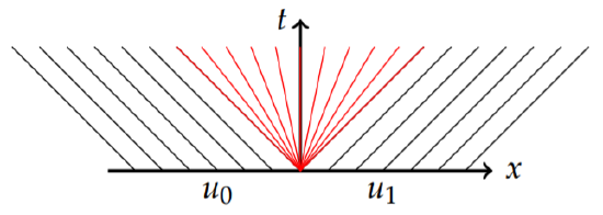
This is a simple model of one-dimensional traffic flow. Let \(u(x, t)\) be the density of cars. Assume that there is no source term. For example, there is no way for a car to disappear from the flow by turning off the road or falling into a sinkhole. Also, there is no source of additional cars.
Solution
Let \(\phi (x, t)\) denote the number of cars per hour passing position \(x\) at time \(t\). Note that the units are given by cars/mi times mi/hr. Thus, we can write the flux as \(\phi = uv\), where \(v\) is the velocity of the carts at position \(x\) and time \(t\).
We can now write the equation for the car density,
\[\begin{align}0&=u_t+\phi 'u_x \nonumber \\ &=u_t+v_1\left(1-\frac{2u}{u_1}\right)u_x.\label{eq:4}\end{align}\]
Nonlinear Advection Equations
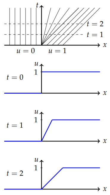
In this section we consider equations of the form \(u_t + c(u)u_x = 0\). When \(c(u)\) is a constant function, we have the advection equation. In the last two examples we have seen cases in which \(c(u)\) is not a constant function. We will apply the method of characteristics to these equations. First, we will recall how the method works for the advection equation.
The advection equation is given by \(u_t + cu_x = 0\). The characteristic equations are given by
\[\frac{dx}{dt}=c,\quad\frac{du}{dt}=0.\nonumber\]
These are easily solved to give the result that
\[u(x,t)=\text{ constant along the lines }x=ct+x_0,\nonumber\]
where \(x_0\) is an arbitrary constant.
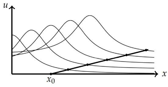
The characteristic lines are shown in Figure \(\PageIndex{3}\). We note that \(u(x, t) = u(x_0, 0) = f(x_0)\). So, if we know \(u\) initially, we can determine what \(u\) is at a later time.
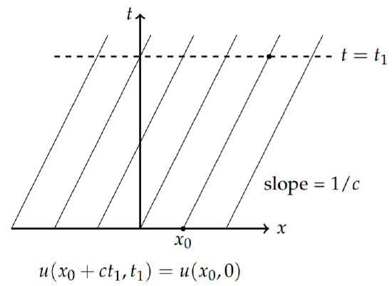
In Figure \(\PageIndex{3}\) we see that the value of \(u(x_0,)\) at \(t = 0\) and \(x = x_0\) propagates along the characteristic to a point at time \(t = t_1\). From \(x − ct = x_0\), we can solve for \(x\) in terms of \(t_1\) and find that \(u(x_0 + ct_1, t_1) = u(x_0, 0)\).
Plots of solutions \(u(x, t)\) versus \(x\) for specific times give traveling waves as shown in Figure 1.3.1. In Figure \(\PageIndex{4}\) we show how each wave profile for different times are constructed for a given initial condition.
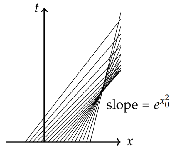
The nonlinear advection equation is given by \(u_t + c(u)u_x = 0\), \(|x| < ∞\). Let \(u(x, 0) = u_0(x)\) be the initial profile. The characteristic equations are given by
\[\frac{dx}{dt}=c(u),\quad\frac{du}{dt}=0.\nonumber\]
These are solved to give the result that
\[u(x,t)=\text{ constant},\nonumber\]
along the characteristic curves \(x'(t) = c(u)\). The lines passing though \(u(x_0,) = u_0(x_0)\) have slope \(1/c(u_0(x_0))\).
Solve \(u_t + uu_x = 0\), \(u(x, 0) = e^{−x^2}\).
Solution
For this problem \(u =\text{ constant}\) along
\[\frac{dx}{dt}=u.\nonumber\]
Since \(u\) is constant, this equation can be integrated to yield \(x = u(x_0, 0)t + x_0\). Inserting the initial condition, \(x = e^{−x^2_0}t + x_0\). Therefore, the solution is
\[u(x,t)=e^{-x^2_0}\text{ along }x=e^{-x^2_0}t+x_0.\nonumber\]
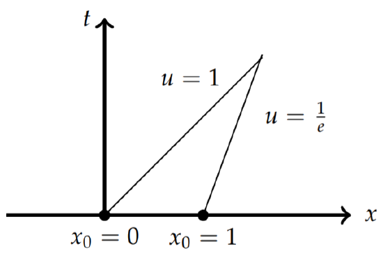
In Figure \(\PageIndex{5}\) the characteristics a shown. In this case we see that the characteristics intersect. In Figure \(\PageIndex{6}\) we look more specifically at the intersection of the characteristic lines for \(x_0 = 0\) and \(x_0 = 1\). These are approximately the first lines to intersect; i.e., there are (almost) no intersections at earlier times. At the intersection point the function \(u(x, t)\) appears to take on more than one value. For the case shown, the solution wants to take the values \(u = 0\) and \(u = 1\).
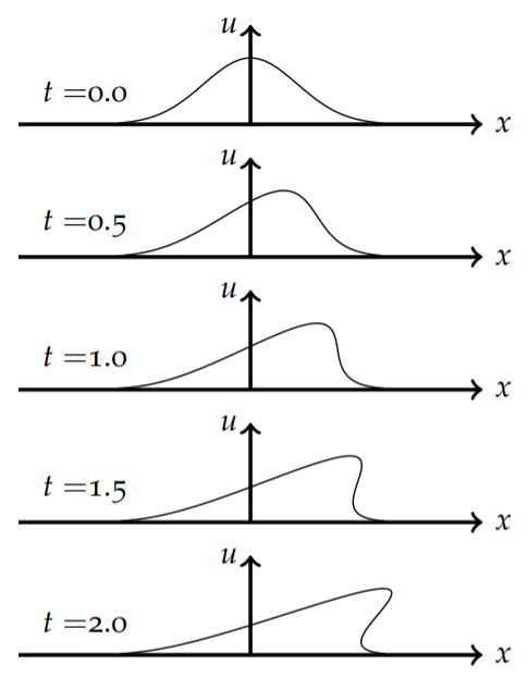
In Figure \(\PageIndex{7}\) we see the development of the solution. This is found using a parametric plot of the points \((x_0 + te^{−x^2_0},e^{−x^2_0})\) for different times. The initial profile propagates to the right with the higher points traveling faster than the lower points since \(x'(t) = u > 0\). Around \(t = 1.0\) the wave breaks and becomes multivalued. The time at which the function becomes multivalued is called the breaking time.
Breaking Time
In the last example we saw that for nonlinear wave speeds a gradient catastrophe might occur. The first time at which a catastrophe occurs is called the breaking time. We will determine the breaking time for the nonlinear advection equation, \(u_t + c(u)u_x = 0\). For the characteristic corresponding to \(x_0 = ξ\), the wavespeed is given by
\[F(\xi )=c(u_0(\xi ))\nonumber\]
and the characteristic line is given by
\[x=\xi +tF(\xi ).\nonumber\]
The value of the wave function along this characteristic is
\[\begin{align}u(x,t)&=u(\xi +tF(\xi ),t)\nonumber \\ &=\: .\label{eq:5}\end{align}\]
Therefore, the solution is
\[u(x, t) = u_0(ξ)\text{ along }x = ξ + tF(ξ).\nonumber\]
This means that
\[u_x =u_0'(\xi)\xi_x\quad\text{and}\quad u_t=u_0'(\xi )\xi_t.\nonumber\]
We can determine \(ξ_x\) and \(ξ_t\) using the characteristic line
\[\xi =x-tF(\xi ).\nonumber\]
Then, we have
\[\begin{align}\xi_x&=1-tF'(\xi )\xi_x \nonumber \\ &=\frac{1}{1+tF'(\xi )}.\nonumber \\ \xi_t&=\frac{\partial}{\partial t}(x-tF(\xi ))\nonumber \\ &=-F(\xi )-tF'(\xi )\xi_t\nonumber \\ &=\frac{-F(\xi)}{1+tF'(\xi)}.\label{eq:6}\end{align}\]
Note that \(ξ_x\) and \(ξ_t\) are undefined if the denominator in both expressions vanishes, \(1 + tF'(ξ) = 0\), or at time
\[t=-\frac{1}{F'(\xi)}.\nonumber\]
The minimum time for this to happen in the breaking time,
\[\label{eq:7}t_b=\text{min}\left\{-\frac{1}{F'(\xi)}\right\}.\]
Find the breaking time for \(u_t + uu_x = 0\), \(u(x, 0) = e^{−x^2}\).
Solution
Since \(c(u) = u\), we have
\[F(\xi)=c(u_0(\xi ))=e^{-\xi^2}\nonumber\]
and
\[F'(\xi )=-2\xi e^{-\xi^2}.\nonumber\]
This goes
\[t=\frac{1}{2\xi e^{-\xi^2}}.\nonumber\]
We need to find the minimum time. Thus, we set the derivative equal to zero and solve for \(ξ\).
\[\begin{align}0&=\frac{d}{d\xi}\left(\frac{e^{\xi^2}}{2\xi}\right)\nonumber \\ &=\left(2-\frac{1}{\xi^2}\right)\frac{e^{\xi^2}}{2}.\label{eq:8}\end{align}\]
Thus, the minimum occurs for \(2 −\frac{1}{\xi^2}= 0\), or \(ξ = 1/\sqrt{2}\). This gives
\[\label{eq:9}t_b=t\left(\frac{1}{\sqrt{2}}\right)=\frac{1}{\frac{2}{\sqrt{2}e^{-1/2}}}=\sqrt{\frac{e}{2}}\approx 1.16.\]
Shock Waves
Solutions of nonlinear advection equations can become multivalued due to a gradient catastrophe. Namely, the derivatives \(u_t\) and \(u_x\) become undefined. We would like to extend solutions past the catastrophe. However, this leads to the possibility of discontinuous solutions. Such solutions which may not be differentiable or continuous in the domain are known as weak solutions. In particular, consider the initial value problem
\[u_t+\phi_x=0,\quad x\in R,\quad t>0,\quad u(x,0)=u_0(x).\nonumber\]
Then, \(u(x, t)\) is a weak solution of this problem if
\[\int_0^\infty \int_{-\infty}^\infty [uv_t+\phi v_x]dxdt+\int_{-\infty}^\infty u_0(x)v(x,0)dx=0\nonumber\]
for all smooth functions \(v ∈ C^∞(R × [0, ∞))\) with compact support, i.e., \(v ≡= 0\) outside some compact subset of the domain.
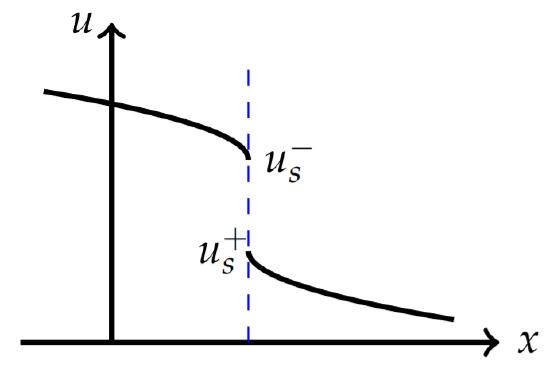
Effectively, the weak solution that evolves will be a piecewise smooth function with a discontinuity, the shock wave, that propagates with shock speed. It can be shown that the form of the shock will be the discontinuity shown in Figure \(\PageIndex{8}\) such that the areas cut from the solutions will cancel leaving the total area under the solution constant. [See G. B. Whitham’s Linear and Nonlinear Waves, 1973.] We will consider the discontinuity as shown in Figure \(\PageIndex{9}\).
We can find the equation for the shock path by using the integral form of the conservation law,
\[\frac{d}{dt}\int_a^b u(x,t)dx=\phi (a,t)-\phi (b,t).\nonumber\]
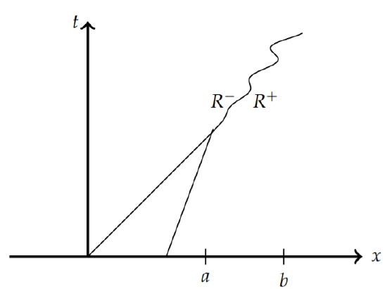
Recall that one can differentiate under the integral if \(u(x, t)\) and \(u_t(x, t)\) are continuous in \(x\) and \(t\) in an appropriate subset of the domain. In particular, we will integrate over the interval \([a, b]\) as shown in Figure \(\PageIndex{10}\). The domains on either side of shock path are denoted as \(R^+\) and \(R^−\) and the limits of \(x(t)\) and \(u(x, t)\) as one approaches from the left of the shock are denoted by \(x_s^− (t)\) and \(u^− = u(x_s^−, t)\). Similarly, the limits of \(x(t)\) and \(u(x, t)\) as one approaches from the right of the shock are denoted by \(x_s^+ (t)\) and \(u^+ = u(x_s^+ , t)\).
We need to be careful in differentiating under the integral,
\[\begin{align}\frac{d}{dt}\int_a^b u(x,t)dx&=\frac{d}{dt}\left[\int_a^{x_s^-(t)}u(x,t)dx+\int_{x_s^+(t)}^bu(x,t)dx\right]\nonumber \\ &=\int_a^{x_s^-(t)}u_t(x,t)dx+\int_{x_s^+(t)}^b u_t(x,t)dx\nonumber \\ &\quad +u(x_s^-,t)\frac{dx_s^-}{dt}-u(x_s^+ ,t)\frac{dx_s^+}{dt}\nonumber \\ &=\phi (a,t)-\phi (b,t).\label{eq:10}\end{align}\]
Taking the limits \(a → x_s^−\) and \(b → x_s^+\), we have that
\[(u(x_s^-,t)-u(x_s^+,t))\frac{dx_s}{dt}=\phi (x_s^-,t)-\phi (x_s^+,t).\nonumber\]
Adopting the notation
\[ [f]=f(x_s^+)-f(x_s^-),\nonumber\]
we arrive at the Rankine-Hugonoit jump condition
\[\label{eq:11}\frac{dx_s}{dt}=\frac{[\phi ]}{[u]}.\]
This gives the equation for the shock path as will be shown in the next example.
Solution
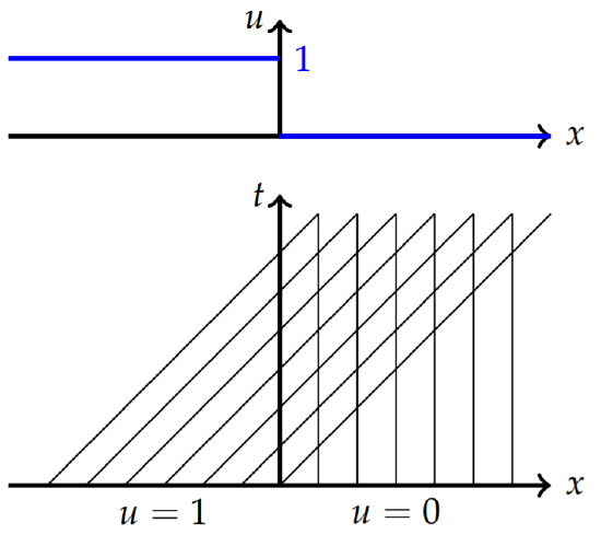
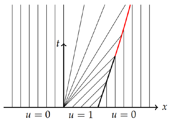
The characteristics for this partial differential equation are familiar by now. The initial condition and characteristics are shown in Figure \(\PageIndex{11}\). From \(x'(t) = u\), there are two possibilities. If \(u = 0\), then we have a constant. If \(u = 1\) along the characteristics, the we have straight lines of slope one. Therefore, the characteristics are given by
\[x(t)=\left\{\begin{array}{cl}x_0,&x>0, \\ t+x_0, &x<0.\end{array}\right.\nonumber\]
As seen in Figure \(\PageIndex{11}\) the characteristics intersect immediately at \(t = 0\). The shock path is found from the Rankine-Hugonoit jump condition. We first note that \(\phi (u) =\frac{1}{2}u^2\), since \(\phi_x = uu_x\). Then, we have
\[\begin{align}\frac{dx_s}{dt}&=\frac{[\phi ]}{[u]} \nonumber \\ &=\frac{\frac{1}{2}u^{+^2}-\frac{1}{2}u^{-^2}}{u^+-u^-} \nonumber \\ &=\frac{1}{2}\frac{(u^++u^-)(u^+-u^-)}{u^+-u^-} \nonumber \\ &=\frac{1}{2}(u^++u^-)\nonumber\\ \label{eq:12}&=\frac{1}{2}(0+1)=\frac{1}{2}.\end{align}\]
Now we need only solve the ordinary differential equation \(x_s' (t) =\frac{1}{2}\) with initial condition \(x_s(0) = 0\). This gives \(x_s(t) =\frac{t}{2}\). This line separates the characteristics on the left and right side of the shock solution. The solution is given by
\[u(x,t)=\left\{\begin{array}{ll}1,&x\leq t/2,\\ 0,&x>t/2.\end{array}\right.\nonumber\]
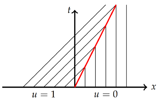
In Figure \(\PageIndex{2}\) we show the characteristic lines ending at the shock path (in red) with \(u = 0\) and on the right and \(u = 1\) on the left of the shock path. This is consistent with the solution. One just sees the initial step function moving to the right with speed \(1/2\) without changing shape
Rarefaction Waves
Shocks are not the only type of solutions encountered when the velocity is a function of \(u\). There may sometimes be regions where the characteristic lines do not appear. A simple example is the following.
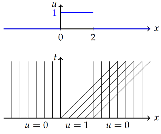
Draw the characteristics for the problem \(u_t + uu_x = 0\), \(|x| < ∞\), \(t > 0\) satisfying the initial condition
\[u(x,0)=\left\{\begin{array}{ll}0,&x\leq 0, \\ 1,&x>0.\end{array}\right.\nonumber\]
Solution
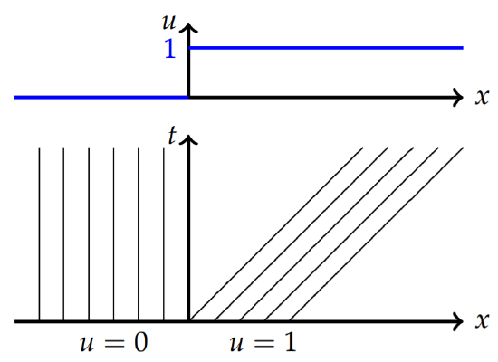
In this case the solution is zero for negative values of \(x\) and positive for positive values of \(x\) as shown in Figure \(\PageIndex{13}\). Since the wavespeed is given by \(u\), the \(u = 1\) initial values have the waves on the right moving to the right and the values on the left stay fixed. This leads to the characteristics in Figure \(\PageIndex{13}\) showing a region in the \(xt\)-plane that has no characteristics. In this section we will discover how to fill in the missing characteristics and, thus, the details about the solution between the \(u = 0\) and \(u = 1\) values.
As motivation, we consider a smoothed out version of this problem.
Draw the characteristics for the initial condition
\[u(x,0)=\left\{\begin{array}{cc} 0, &x\leq -\epsilon , \\ \frac{x+\epsilon}{2\epsilon},&|x|\leq\epsilon , \\ 1,&x>\epsilon.\end{array}\right.\nonumber\]
Solution
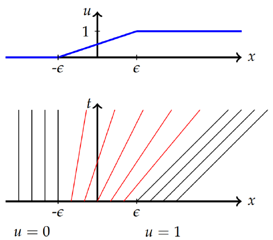
The function is shown in the top graph in Figure \(\PageIndex{14}\). The leftmost and rightmost characteristics are the same as the previous example. The only new part is determining the equations of the characteristics for \(|x| ≤\epsilon\). These are found using the method of characteristics as
\[x=\xi +u_0(\xi )t,\quad u_0(\xi )=\frac{\xi+\epsilon}{2\epsilon}t.\nonumber\]
These characteristics are drawn in Figure \(\PageIndex{14}\) in red. Note that these lines take on slopes varying from infinite slope to slope one, corresponding to speeds going from zero to one.
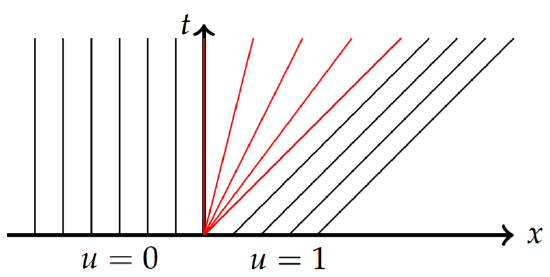
Comparing the last two examples, we see that as \(\epsilon\) approaches zero, the last example converges to the previous example. The characteristics in the region where there were none become a “fan”. We can see this as follows. Since \(|ξ| <\epsilon\) for the fan region, as \(\epsilon\) gets small, so does this interval. Let’s scale \(ξ\) as \(ξ = σ\epsilon\), \(σ ∈ [−1, 1]\). Then,
\[x=\sigma\epsilon +u_0(\sigma\epsilon )t,\quad u_0(\sigma\epsilon )=\frac{\sigma\epsilon +\epsilon}{2\epsilon}t=\frac{1}{2}(\sigma +1)t.\nonumber\]
For each \(σ ∈ [−1, 1]\) there is a characteristic. Letting \(\epsilon → 0\), we have
\[x=ct,\quad c=\frac{1}{2}(\sigma +1)t.\nonumber\]
Thus, we have a family of straight characteristic lines in the \(xt\)-plane passing through \((0, 0)\) of the form \(x = ct\) for \(c\) varying from \(c = 0\) to \(c = 1\). These are shown as the red lines in Figure \(\PageIndex{15}\).
The fan characteristics can be written as \(x/t =\) constant. So, we can seek to determine these characteristics analytically and in a straight forward manner by seeking solutions of the form \(u(x, t) = g\left(\frac{x}{t}\right)\).
Determine solutions of the form \(u(x, t) = g\left(\frac{x}{t}\right)\) to \(u_t + uu_x = 0\). Inserting this guess into the differential equation, we have
\[\begin{align}0&=u_t+uu_x \nonumber \\ &=\frac{1}{t}g'\left(g-\frac{x}{t}\right).\label{eq:13}\end{align}\]
Solution
Thus, either \(g' = 0\) or \(g =\frac{x}{t}\). The first case will not work since this gives constant solutions. The second solution is exactly what we had obtained before. Recall that solutions along characteristics give \(u(x, t) = \frac{x}{t} =\text{ constant}\). The characteristics and solutions for \(t = 0, 1, 2\) are shown in Figure \(\PageIndex{16}\). At a specific time one can draw a line (dashed lines in figure) and follow the characteristics back to the \(t = 0\) values, \(u(ξ, 0)\) in order to construct \(u(x, t)\).
As a last example, let’s investigate a nonlinear model which possesses both shock and rarefaction waves.
Solve the initial value problem \(u_t + u^2u_x = 0\), \(|x| < ∞\), \(t > 0\) satisfying the initial condition
\[u(x,0)=\left\{\begin{array}{lc}0,&x\leq 0, \\ 1,&0<x<2, \\ 0,&x\geq 2.\end{array}\right.\nonumber\]
Solution
The method of characteristics gives
\[\frac{dx}{dt}=u^2,\quad \frac{du}{dt}=0.\nonumber\]
Therefore,
\[u(x,t)=u_0(\xi)=\text{ const. along the lines }x(t)=u_0^2(\xi )t+\xi .\nonumber\]
There are three values of \(u_0(ξ)\),
\[u_0(\xi )=\left\{\begin{array}{lc}0,&\xi\leq 0, \\ 1,& 0<\xi <2, \\ 0, &\xi\geq 2.\end{array}\right.\nonumber\]
In Figure \(\PageIndex{17}\) we see that there is a rarefaction and a gradient catastrophe.
Therefore, along the fan characteristics the solutions are \(u(x, t) =\sqrt{\frac{x}{t}} =\text{ constant}.\) These fan characteristics are added in Figure \(\PageIndex{18}\).
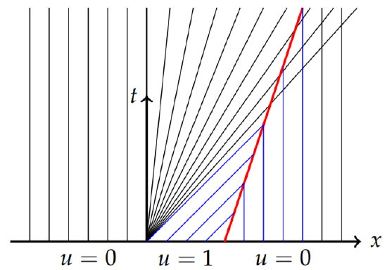
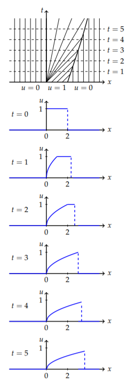
Next, we turn to the shock path. We see that the first intersection occurs at the point \((x, t) = (2, 0)\). The Rankine-Hugonoit condition gives
\[\begin{align}\frac{dx_s}{dt}&=\frac{[\phi ]}{[u]}\nonumber \\ &=\frac{\frac{1}{2}u^{+^3}-\frac{1}{3}u^{-^3}}{u^+-u^-} \nonumber \\ &=\frac{1}{3}\frac{(u^+-u^-)(u^{+^2}+u^+u^-+u^{-^2})}{u^+-u^-}\nonumber \\ &=\frac{1}{3}(u^{+^2}+u^+u^-+u^{-^2}\nonumber \\ &=\frac{1}{3}(0+0+1)=\frac{1}{3}.\label{eq:15}\end{align}\]
Thus, the shock path is given by \(x_s' (t) =\frac{1}{3}\) with initial condition \(x_s(0) = 2\). This gives \(x_s(t) = \frac{t}{3}+ 2\). In Figure \(\PageIndex{19}\) the shock path is shown in red with the fan characteristics and vertical lines meeting the path. Note that the fan lines and vertical lines cross the shock path. This leads to a change in the shock path.
The new path is found using the Rankine-Hugonoit condition with \(u^+ = 0\) and \(u^− =\sqrt{\frac{x}{t}}\). Thus,
\[\begin{align}\frac{dx_s}{dt}&=\frac{[\phi]}{[u]}\nonumber \\ &=\frac{\frac{1}{3}u^{+^3}-\frac{1}{3}u^{-^3}}{u^+-u^-} \nonumber \\ &=\frac{1}{3}\frac{(u^+-u^-)(u^{+^2}+u^+u^-+u^{-^2})}{u^+-u^-} \nonumber \\ &=\frac{1}{3}(u^{+^2}+u^+u^-+u^{-^2})\nonumber \\ &=\frac{1}{3}(0+0+\sqrt{\frac{x_s}{t}})=\frac{1}{3}\sqrt{\frac{x_s}{t}}.\label{eq:16}\end{align}\]
We need to solve the initial value problem
\[\frac{dx_s}{dt}=\frac{1}{3}\sqrt{\frac{x_s}{t}},\quad x_s(3)=3.\nonumber\]
This can be done using separation of variables. Namely,
\[\int\frac{dx_s}{\sqrt{x_s}}=\frac{1}{3}\frac{t}{\sqrt{t}}.\nonumber\]
This gives the solution
\[\sqrt{x_s}=\frac{1}{3}\sqrt{t}+c.\nonumber\]
Since the second shock solution starts at the point \((3, 3)\), we can determine \(c =\frac{2}{3}\sqrt{3}\). This gives the shock path as
\[x_s(t)=\left(\frac{1}{3}\sqrt{t}+\frac{2}{3}\sqrt{3}\right)^2.\nonumber\]
In Figure \(\PageIndex{20}\) we show this shock path and the other characteristics ending on the path.
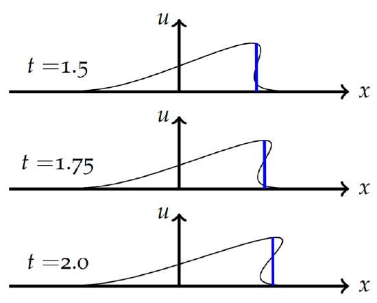
It is interesting to construct the solution at different times based on the characteristics. For a given time, \(t\), one draws a horizontal line in the \(xt\)-plane and reads off the values of \(u(x, t)\) using the values at \(t = 0\) and the rarefaction solutions. This is shown in Figure \(\PageIndex{21}\). The right discontinuity in the initial profile continues as a shock front until \(t = 3\). At that time the back rarefaction wave has caught up to the shock. After \(t = 3\), the shock propagates forward slightly slower and the height of the shock begins to decrease. Due to the fact that the partial differential equation is a conservation law, the area under the shock remains constant as it stretches and decays in amplitude.
Traffic Flow
An interesting application is that of traffic flow. We had already derived the flux function. Let’s investigate examples with varying initial conditions that lead to shock or rarefaction waves. As we had seen earlier in modeling traffic flow, we can consider the flux function
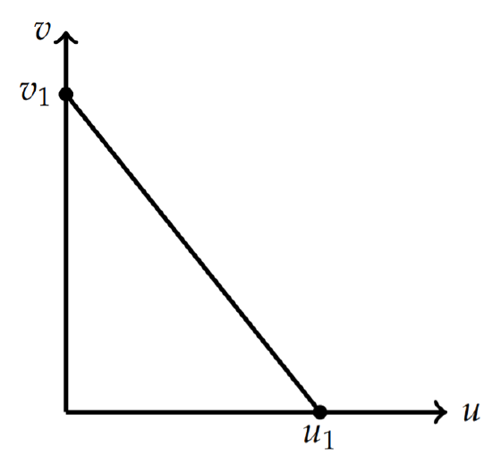
\[\phi =uv=v_1\left(u-\frac{u^2}{u_1}\right),\nonumber\]
which leads to the conservation law
\[u_t+v_1(1-\frac{2u}{u_1})u_x=0.\nonumber\]
Here \(u(x, t)\) represents the density of the traffic and \(u_1\) is the maximum density and \(v_1\) is the initial velocity.
The characteristics for this problem are given by
\[x=c(u(x_0,t))t+x_0,\nonumber\]
where
\[x(u(x_0,t))=v_1(1-\frac{2u(x_0,0)}{u_1}).\nonumber\]
Since the initial condition is a piecewise-defined function, we need to consider two cases.
First, for \(x ≥ 0\), we have
\[c(u(x_0,t))=c(u_1)=v_1(1-\frac{2u_1}{u_1})=-v_1.\nonumber\]
Therefore, the slopes of the characteristics, \(x = −v_1t + x_0\) are \(−1/v_1\).
For \(x_0 < 0\), we have
\[c(u(x_0,t))=c(u_0)=v_1(1-\frac{2u_0}{u_1}).\nonumber\]
So, the characteristics are \(x = −v_1(1 −\frac{2u_0}{u_1})t + x_0\).
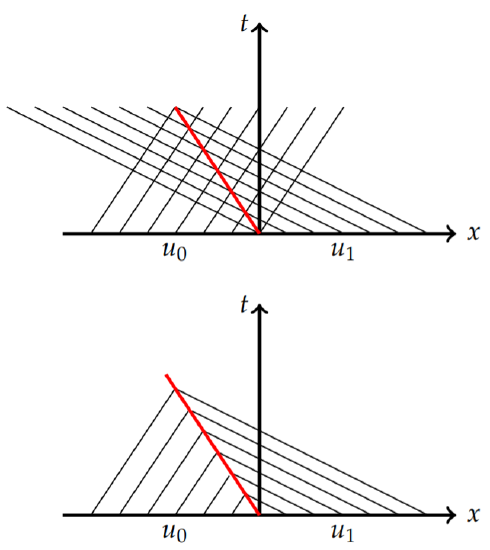
In Figure \(\PageIndex{23}\) we plot the initial condition and the characteristics for \(x < 0\) and \(x > 0\). We see that there are crossing characteristics and the begin crossing at \(t = 0\). Therefore, the breaking time is \(t_b = 0\). We need to find the shock path satisfying \(x_s(0) = 0\). The Rankine-Hugonoit conditions give
\[\begin{align}\frac{dx_s}{dt}&=\frac{[\phi]}{[u]}\nonumber \\ &=\frac{\frac{1}{2}u^{+^2}-\frac{1}{2}u^{-^2}}{u^+-u^-}\nonumber \\ &=\frac{1}{2}\frac{0-v_1\frac{u_0^2}{u_1}}{u_1-u_0}\nonumber \\ &=-v_1\frac{u_0}{u_1}.\label{eq:17}\end{align}\]
Thus, the shock path is found as \(x_s(t) = −v_1\frac{u_0}{u_1}\).
In Figure \(\PageIndex{24}\) we show the shock path. In the top figure the red line shows the path. In the lower figure the characteristics are stopped on the shock path to give the complete picture of the characteristics. The picture was drawn with \(v_1 = 2\) and \(u_0/u_1 = 1/3\).
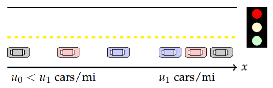
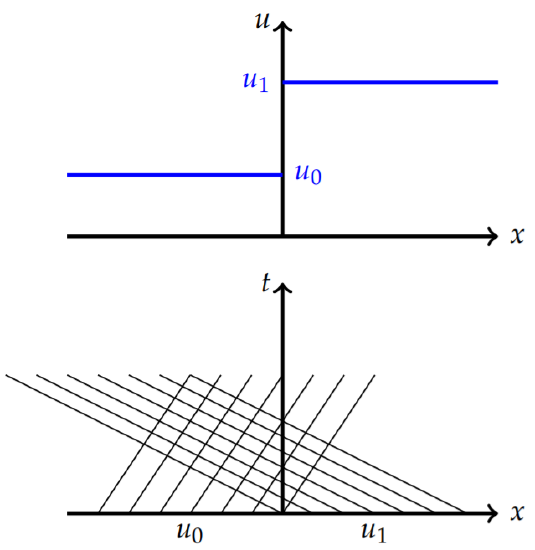
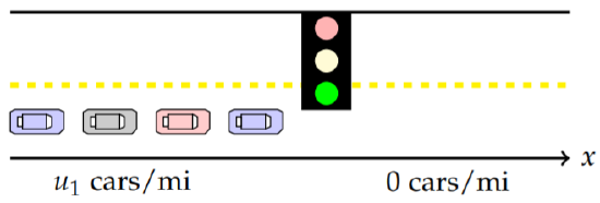
The next problem to consider is stopped traffic as the light turns green. The cars in Figure \(\PageIndex{25}\) begin to fan out when the traffic light turns green. In this model the initial condition is given by
\[u(x,0)=\left\{\begin{array}{cc}u_1,&x\leq 0, \\ 0, & x>0.\end{array}\right.\nonumber\]
Again,
\[c(u(x_0, t))=v_1(1-\frac{2u(x_0,0)}{u_1}).\nonumber\]
Inserting the initial values of \(u\) into this expression, we obtain constant speeds, \(±v_1\). The resulting characteristics are given by
\[x(t)=\left\{\begin{array}{cc}-v_1t+x_0, &x\leq 0, \\ v_1t+x_0, &x>0.\end{array}\right.\nonumber\]