
3.1: Introduction to Fourier Series
- Page ID
- 90251

We will now turn to the study of trigonometric series. You have seen that functions have series representations as expansions in powers of \(x\), or \(x − a\), in the form of Maclaurin and Taylor series. Recall that the Taylor series expansion is given by
\[f(x)=\sum\limits_{n=0}^\infty c_n(x-a)^n,\nonumber\]
where the expansion coefficients are determined as
\[c_n=\frac{f^{(n)}(a)}{n!}.\nonumber\]
From the study of the heat equation and wave equation, we have found that there are infinite series expansions over other functions, such as sine functions. We now turn to such expansions and in the next chapter we will find out that expansions over special sets of functions are not uncommon in physics. But, first we turn to Fourier trigonometric series.
We will begin with the study of the Fourier trigonometric series expansion
\[f(x)=\frac{a_0}{2}+\sum\limits_{n=1}^\infty a_n\cos\frac{n\pi x}{L}+b_n\sin\frac{n\pi x}{L}.\nonumber\]
We will find expressions useful for determining the Fourier coefficients \(\{a_n, b_n\}\) given a function \(f(x)\) defined on \([−L, L]\). We will also see if the resulting infinite series reproduces \(f(x)\). However, we first begin with some basic ideas involving simple sums of sinusoidal functions.
There is a natural appearance of such sums over sinusoidal functions in music. A pure note can be represented as
\[y(t)=A\sin (2\pi ft),\nonumber\]
where \(A\) is the amplitude, \(f\) is the frequency in hertz (Hz), and \(t\) is time in seconds. The amplitude is related to the volume of the sound. The larger the amplitude, the louder the sound. In Figure \(\PageIndex{2}\) we show plots of two such tones with \(f = 2\text{ Hz}\) in the top plot and \(f = 5\text{ Hz}\) in the bottom one.
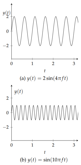
In these plots you should notice the difference due to the amplitudes and the frequencies. You can easily reproduce these plots and others in your favorite plotting utility.
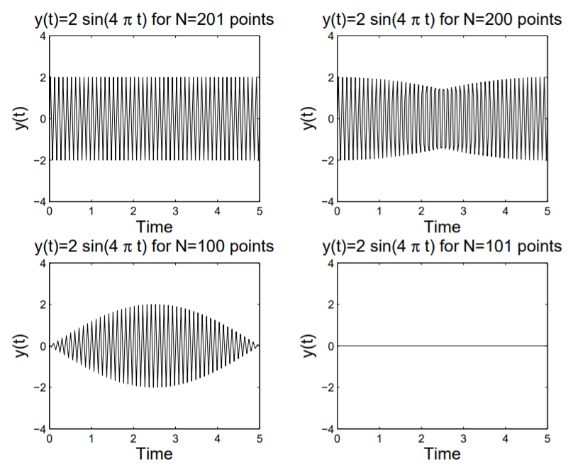
As an aside, you should be cautious when plotting functions, or sampling data. The plots you get might not be what you expect, even for a simple sine function. In Figure \(\PageIndex{2}\) we show four plots of the function \(y(t) = 2 \sin(4πt)\). In the top left you see a proper rendering of this function. However, if you use a different number of points to plot this function, the results may be surprising. In this example we show what happens if you use \(N = 200, 100, 101\) points instead of the \(201\) points used in the first plot. Such disparities are not only possible when plotting functions, but are also present when collecting data. Typically, when you sample a set of data, you only gather a finite amount of information at a fixed rate. This could happen when getting data on ocean wave heights, digitizing music and other audio to put on your computer, or any other process when you attempt to analyze a continuous signal.
Next, we consider what happens when we add several pure tones. After all, most of the sounds that we hear are in fact a combination of pure tones with different amplitudes and frequencies. In Figure \(\PageIndex{3}\) we see what happens when we add several sinusoids. Note that as one adds more and more tones with different characteristics, the resulting signal gets more complicated. However, we still have a function of time. In this chapter we will ask, “Given a function \(f(t)\), can we find a set of sinusoidal functions whose sum converges to \(f(t)\)?”
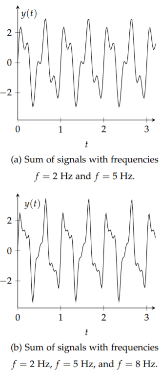
Looking at the superpositions in Figure \(\PageIndex{3}\), we see that the sums yield functions that appear to be periodic. This is not to be unexpected. We recall that a periodic function is one in which the function values repeat over the domain of the function. The length of the smallest part of the domain which repeats is called the period. We can define this more precisely: A function is said to be periodic with period \(T\) if \(f(t + T) = f(t)\) for all \(t\) and the smallest such positive number \(T\) is called the period.
For example, we consider the functions used in Figure \(\PageIndex{3}\). We began with \(y(t) = 2 \sin(4πt)\). Recall from your first studies of trigonometric functions that one can determine the period by dividing the coefficient of \(t\) into \(2π\) to get the period. In this case we have
\[T=\frac{2\pi}{4\pi}=\frac{1}{2}.\nonumber\]
Looking at the top plot in Figure \(\PageIndex{1}\) we can verify this result. (You can count the full number of cycles in the graph and divide this into the total time to get a more accurate value of the period.)
In general, if \(y(t) = A \sin(2π f t)\), the period is found as
\[T=\frac{2\pi}{2\pi f}=\frac{1}{f}.\nonumber\]
Of course, this result makes sense, as the unit of frequency, the hertz, is also defined as \(s^{−1}\), or cycles per second.
Returning to Figure \(\PageIndex{3}\), the functions \(y(t) = 2 \sin(4πt)\), \(y(t) = \sin(10πt)\), and \(y(t) = 0.5 \sin(16πt)\) have periods of \(0.5\text{s},\: 0.2\text{s}\), and \(0.125\text{s}\), respectively. Each superposition in Figure \(\PageIndex{3}\) retains a period that is the least common multiple of the periods of the signals added. For both plots, this is \(1.0\text{s} = 2(0.5)\text{s} = 5(.2)\text{s} = 8(.125)\text{s}\).
Our goal will be to start with a function and then determine the amplitudes of the simple sinusoids needed to sum to that function. We will see that this might involve an infinite number of such terms. Thus, we will be studying an infinite series of sinusoidal functions.
Secondly, we will find that using just sine functions will not be enough either. This is because we can add sinusoidal functions that do not necessarily peak at the same time. We will consider two signals that originate at different times. This is similar to when your music teacher would make sections of the class sing a song like “Row, Row, Row your Boat” starting at slightly different times.
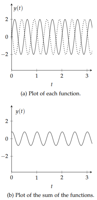
We can easily add shifted sine functions. In Figure \(\PageIndex{4}\) we show the functions \(y(t) = 2 \sin(4πt)\) and \(y(t) = 2 \sin(4πt + 7π/8)\) and their sum. Note that this shifted sine function can be written as \(y(t) = 2 \sin(4π(t + 7/32))\). Thus, this corresponds to a time shift of \(−7/32\).
So, we should account for shifted sine functions in the general sum. Of course, we would then need to determine the unknown time shift as well as the amplitudes of the sinusoidal functions that make up the signal, \(f(t)\). While this is one approach that some researchers use to analyze signals, there is a more common approach. This results from another reworking of the shifted function.
We should note that the form in the lower plot of Figure 3.4 looks like a simple sinusoidal function for a reason. Let
\[y_1(t)=2\sin (4\pi t),\nonumber \]
\[y_2(t)=2\sin (4\pi t+7\pi /8).\nonumber\]
Then,
\[\begin{aligned} y_1+y_2&=2 \sin(4πt + 7π/8) + 2 \sin(4πt) \\ & = 2[\sin(4πt + 7π/8) + \sin(4πt)] \\ &=4\cos\frac{7\pi}{16}\sin\left( 4\pi t+\frac{7\pi}{16}\right).\end{aligned}\]
[1] Recall the identities (11.2.5)-(11.2.6)
\[\begin{aligned}\sin(x+y)&=\sin x\cos y+\sin y\cos x, \\ \cos(x+y)&=\cos x\cos y-\sin x\sin y.\end{aligned}\]
Consider the general shifted function
\[y(t)=A\sin (2\pi ft+\phi ).\label{eq:1}\]
Note that \(2\pi f t +\phi\) is called the phase of the sine function and \(\phi\) is called the phase shift. We can use the trigonometric identity (A.17) for the sine of the sum of two angles\(^{1}\) to obtain
\[\begin{align} y(t)&=A\sin (2\pi ft+\phi )\nonumber \\ &=A\sin (\phi )\cos (2\pi ft)+A\cos (\phi )\sin (2\pi ft).\label{eq:2}\end{align}\]
We are now in a position to state our goal.
Given a signal \(f(t)\), we would like to determine its frequency content by finding out what combinations of sines and cosines of varying frequencies and amplitudes will sum to the given function. This is called Fourier Analysis.