3.3: Fourier Series Over Other Intervals

In many applications we are interested in determining Fourier series representations of functions defined on intervals other than \([0, 2π]\). In this section we will determine the form of the series expansion and the Fourier coefficients in these cases.

The most general type of interval is given as \([a, b]\). However, this often is too general. More common intervals are of the form \([−π, π],\: [0, L],\) or \([−L/2, L/2]\). The simplest generalization is to the interval \([0, L]\). Such intervals arise often in applications. For example, for the problem of a one dimensional string of length \(L\) we set up the axes with the left end at \(x = 0\) and the right end at \(x = L\). Similarly for the temperature distribution along a one dimensional rod of length \(L\) we set the interval to \(x ∈ [0, 2π]\). Such problems naturally lead to the study of Fourier series on intervals of length \(L\). We will see later that symmetric intervals, \([−a, a]\), are also useful.

Given an interval \([0, L]\), we could apply a transformation to an interval of length \(2π\) by simply rescaling the interval. Then we could apply this transformation to the Fourier series representation to obtain an equivalent one useful for functions defined on \([0, L]\).

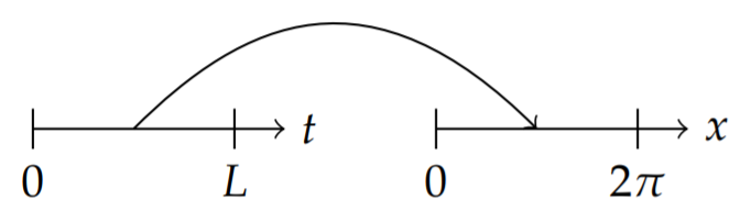
We define \(x ∈ [0, 2π]\) and \(t ∈ [0, L]\). A linear transformation relating these intervals is simply \(x = \frac{2πt}{L}\) as shown in Figure \(\PageIndex{1}\). So, \(t = 0\) maps to \(x = 0\) and \(t = L\) maps to \(x = 2π\). Furthermore, this transformation maps \(f(x)\) to a new function \(g(t) = f(x(t))\), which is defined on \([0, L]\). We will determine the Fourier series representation of this function using the representation for \(f(x)\) from the last section.

Figure \(\PageIndex{1}\): A sketch of the transformation between intervals \(x ∈ [0, 2π]\) and \(t ∈ [0, L]\).

Recall the form of the Fourier representation for \(f(x)\) in Equation (3.2.1):

\[\label{eq:1} f(x)\sim\frac{a_0}{2}+\sum\limits_{n=1}^\infty [a_n\cos nx+b_n\sin nx].\]

Inserting the transformation relating \(x\) and \(t\), we have

\[\label{eq:2}g(t)\sim\frac{a_0}{2}+\sum\limits_{n=1}^\infty\left[a_n\cos\frac{2n\pi t}{L}+b_n\sin\frac{2n\pi t}{L}\right].\]

This gives the form of the series expansion for \(g(t)\) with \(t ∈ [0, L]\). But, we still need to determine the Fourier coefficients.

Recall, that

\[a_n=\frac{1}{\pi}\int_0^{2\pi}f(x)\cos nxdx.\nonumber\]

We need to make a substitution in the integral of \(x = \frac{2πt}{L}\). We also will need to transform the differential, \(dx = \frac{2π}{L} dt\). Thus, the resulting form for the Fourier coefficients is

\[\label{eq:3}a_n=\frac{2}{L}\int_0^L g(t)\cos\frac{2n\pi t}{L}dt.\]

Similarly, we find that

\[\label{eq:4}b_n=\frac{2}{L}\int_0^L g(t)\sin\frac{2n\pi t}{L}dt.\]

We note first that when \(L = 2π\) we get back the series representation that we first studied. Also, the period of \(\cos \frac{2nπt}{L}\) is \(L/n\), which means that the representation for \(g(t)\) has a period of \(L\) corresponding to \(n = 1\).

At the end of this section we present the derivation of the Fourier series representation for a general interval for the interested reader. In Table \(\PageIndex{1}\) we summarize some commonly used Fourier series representations.

Table \(\PageIndex{1}\): Special Fourier Series Representations on Different Intervals

Fourier Series on \([0,L]\)
\[\label{eq:5}f(x)\sim\frac{a_0}{2}+\sum\limits_{n=1}^\infty\left[a_n\cos\frac{2n\pi x}{L}+b_n\sin\frac{2n\pi x}{L}\right].\]
\[\begin{align}a_n&=\frac{2}{L}\int_0^Lf(x)\cos\frac{2n\pi x}{L}dx.\quad n=0,1,2,\ldots ,\nonumber \\ b_n&=\frac{2}{L}\int_0^L f(x)\sin\frac{2n\pi x}{L}dx.\quad n=1,2,\ldots .\label{eq:6}\end{align}\]
Fourier Series on \([-\frac{L}{2},\frac{L}{2}]\)
\[\label{eq:7}f(x)\sim\frac{a_0}{2}+\sum\limits_{n=1}^\infty\left[a_n\cos\frac{2n\pi x}{L}+b_n\sin\frac{2n\pi x}{L}\right].\]
\[\begin{align}a_n&=\frac{2}{L}\int_{-\frac{L}{2}}^{\frac{L}{2}}f(x)\cos\frac{2n\pi x}{L}dx.\quad n=0,1,2,\ldots ,\nonumber \\ b_n&=\frac{2}{L}\int_{-\frac{L}{2}}^{\frac{L}{2}} f(x)\sin\frac{2n\pi x}{L}dx.\quad n=1,2,\ldots .\label{eq:8}\end{align}\]
Fourier Series on \([-\pi ,\pi ]\)
\[\label{eq:9}f(x)\sim\frac{a_0}{2}+\sum\limits_{n=1}^\infty [a_n\cos nx+b_n\sin nx].\]
\[\begin{align}a_n&=\frac{1}{\pi}\int_{-\pi}^\pi f(x)\cos nxdx.\quad n=0,1,2,\ldots ,\nonumber \\ b_n&=\frac{1}{\pi}\int_{-\pi}^\pi f(x)\sin nxdx.\quad n=1,2,\ldots .\label{eq:10}\end{align}\]

At this point we need to remind the reader about the integration of even and odd functions on symmetric intervals.

We first recall that \(f(x)\) is an even function if \(f(−x) = f(x)\) for all \(x\). One can recognize even functions as they are symmetric with respect to the \(y\)-axis as shown in Figure \(\PageIndex{2}\).

Figure \(\PageIndex{2}\): Area under an even function on a symmetric interval, \([−a, a]\).

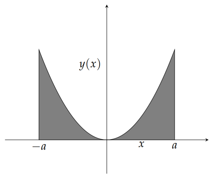
If one integrates an even function over a symmetric interval, then one has that

\[\label{eq:11}\int_{-a}^af(x)dx=2\int_0^af(x)dx.\]

One can prove this by splitting off the integration over negative values of \(x\), using the substitution \(x = −y\), and employing the evenness of \(f(x)\). Thus,

\[\begin{align}\int_{-a}^af(x)dx&=\int_{-a}^0f(x)dx+\int_0^af(x)dx\nonumber \\ &=-\int_a^0f(-y)dy+\int_0^af(x)dx\nonumber \\ &=\int_0^af(y)dy+\int_0^af(x)dx\nonumber \\ &=2\int_0^af(x)dx.\label{eq:12}\end{align}\]

This can be visually verified by looking at Figure \(\PageIndex{2}\).

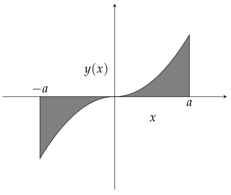
A similar computation could be done for odd functions. \(f(x)\) is an odd function if \(f(−x) = −f(x)\) for all \(x\). The graphs of such functions are symmetric with respect to the origin as shown in Figure \(\PageIndex{3}\). If one integrates an odd function over a symmetric interval, then one has that

\[\label{eq:13}\int_{-a}^af(x)dx=0.\]

Figure \(\PageIndex{3}\): Area under an odd function on a symmetric interval, \([−a, a]\).

Example \(\PageIndex{1}\)

Let \(f(x) = |x|\) on \([−π, π]\). We compute the coefficients, beginning as usual with \(a_0\). We have, using the fact that \(|x|\) is an even function,

\[\begin{align}a_0&=\frac{1}{\pi}\int_{-\pi}^\pi |x|dx\nonumber \\ &=\frac{2}{\pi}\int_0^{\pi}xdx=\pi\label{eq:14}\end{align}\]

We continue with the computation of the general Fourier coefficients for \(f(x) = |x|\) on \([−π, π]\). We have

\[\label{eq:15}a_n=\frac{1}{\pi}\int_{-\pi}^\pi |x|\cos nxdx=\frac{2}{\pi}\int_0^{\pi}x\cos nxdx.\]

Here we have made use of the fact that \(|x| \cos nx\) is an even function.

In order to compute the resulting integral, we need to use integration by parts,

\[\int_a^b udv=\left. uv\right|_a^b-\int_a^b vdu,\nonumber\]

by letting \(u = x\) and \(dv = \cos nx dx\). Thus, \(du = dx\) and \(v = \int dv = \frac{1}{n}\sin nx\).

Continuing with the computation, we have

\[\begin{align}a_n&=\frac{2}{\pi}\int_0^\pi x\cos nxdx.\nonumber \\ &=\frac{2}{\pi}\left[\frac{1}{n}x\sin nx \right|_0^\pi -\left.\frac{1}{n}\int_0^\pi \sin nxdx\right] \nonumber \\ &=-\frac{2}{n\pi}\left[-\frac{1}{n}\cos nx\right]_0^\pi\nonumber \\ &=-\frac{2}{\pi n^2}(1-(-1)^n).\label{eq:16}\end{align}\]

Here we have used the fact that \(\cos nπ = (−1)^n\) for any integer \(n\). This leads to a factor \((1 − (−1)^n )\). This factor can be simplified as

\[\label{eq:17}1-(-1)^n=\left\{\begin{array}{rl}2,&n\text{ odd} \\ 0,&n\text{ even}\end{array}\right. .\]

So, \(a_n = 0\) for \(n\) even and \(a_n = −\frac{4}{\pi n^2}\) for \(n\) odd.

Computing the \(b_n\)’s is simpler. We note that we have to integrate \(|x| \sin nx\) from \(x = −π\) to \(π\). The integrand is an odd function and this is a symmetric interval. So, the result is that \(b_n = 0\) for all \(n\).

Putting this all together, the Fourier series representation of \(f(x) = |x|\) on \([−π, π]\) is given as

\[\label{eq:18}f(x)\sim\frac{\pi}{2}-\frac{4}{\pi}\sum\limits_{\underset{n\text{ odd}}{n=1}}^\infty \frac{\cos nx}{n^2}.\]

While this is correct, we can rewrite the sum over only odd n by reindexing. We let \(n = 2k − 1\) for \(k = 1, 2, 3,\ldots\). Then we only get the odd integers. The series can then be written as

\[\label{eq:19}f(x)\sim\frac{\pi}{2}-\frac{4}{\pi}\sum\limits_{k=1}^\infty\frac{\cos (2k-1)x}{(2k-1)^2}.\]

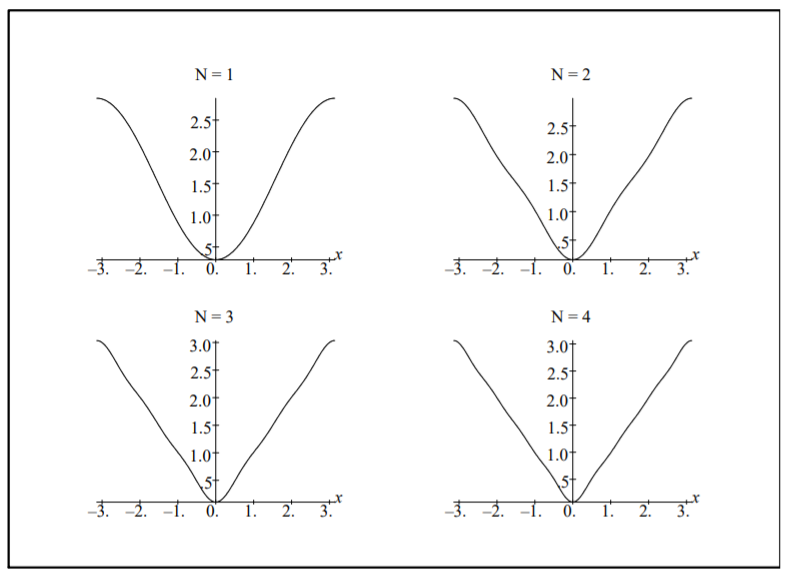
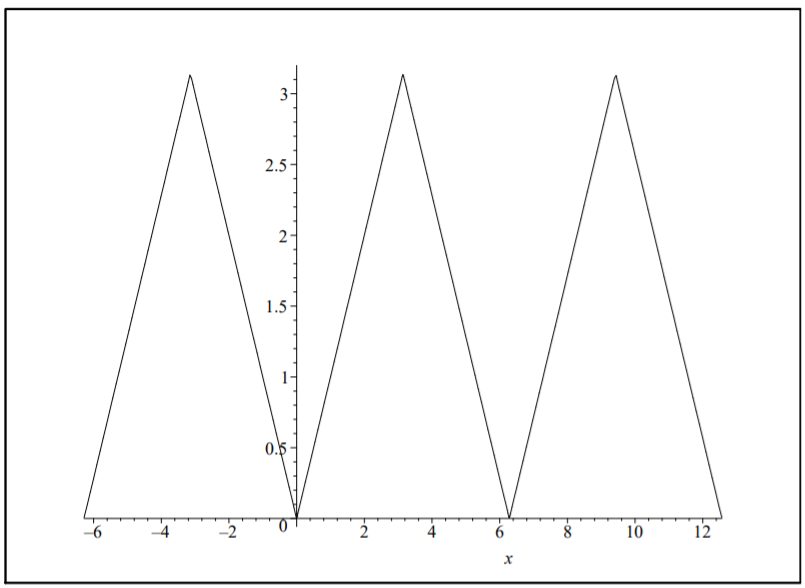
Throughout our discussion we have referred to such results as Fourier representations. We have not looked at the convergence of these series. Here is an example of an infinite series of functions. What does this series sum to? We show in Figure \(\PageIndex{4}\) the first few partial sums. They appear to be converging to \(f(x) = |x|\) fairly quickly.

Figure \(\PageIndex{4}\): Plot of the first partial sums of the Fourier series representation for \(f(x) = |x|\).

Even though \(f(x)\) was defined on \([−π, π]\) we can still evaluate the Fourier series at values of \(x\) outside this interval. In Figure \(\PageIndex{5}\), we see that the representation agrees with \(f(x)\) on the interval \([−π, π]\). Outside this interval we have a periodic extension of \(f(x)\) with period \(2π\).

Figure \(\PageIndex{5}\): Plot of the first 10 terms of the Fourier series representation for \(f(x) = |x|\) on the interval \([−2π, 4π]\).

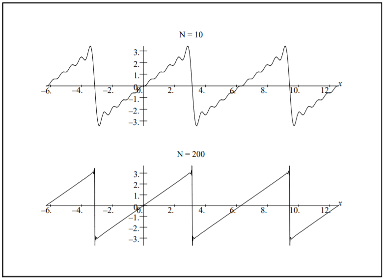
Another example is the Fourier series representation of \(f(x) = x\) on \([−π, π]\) as left for Problem 7. This is determined to be

\[\label{eq:20}f(x)\sim 2\sum\limits_{n=1}^\infty \frac{(-1)^{n+1}}{n}\sin nx.\]

As seen in Figure \(\PageIndex{6}\) we again obtain the periodic extension of the function. In this case we needed many more terms. Also, the vertical parts of the first plot are nonexistent. In the second plot we only plot the points and not the typical connected points that most software packages plot as the default style.

Figure \(\PageIndex{6}\): Plot of the first \(10\) terms and \(200\) terms of the Fourier series representation for \(f(x) = x\) on the interval \([−2π, 4π]\).

Example \(\PageIndex{2}\)

It is interesting to note that one can use Fourier series to obtain sums of some infinite series. For example, in the last example we found that

\[x\sim 2\sum\limits_{n=1}^\infty \frac{(-1)^{n+1}}{n}\sin nx.\nonumber\]

Now, what if we chose \(x =\frac{\pi}{2}\)? Then, we have

\[\frac{\pi}{2}=2\sum\limits_{n=1}^\infty\frac{(-1)^{n+1}}{n}\sin\frac{n\pi}{2}=2\left[1-\frac{1}{3}+\frac{1}{5}-\frac{1}{7}+\cdots\right].\nonumber\]

This gives a well known expression for \(π\):

\[\pi =4\left[1-\frac{1}{3}+\frac{1}{5}-\frac{1}{7}+\cdots\right].\nonumber\]

Fourier Series on \([a,b]\)

A Fourier series representation is also possible for a general interval, \(t\in [a,b]\). As before, we just need to transform this interval to [0, 2π]. Let \[x=2\pi\frac{t-a}{b-a}.\nonumber\]

Inserting this into the Fourier series (3.2.1) representation for \(f(x)\) we obtain \[\label{eq:21}g(t)\sim\frac{a_0}{2}+\sum\limits_{n=1}^\infty\left[a_n\cos\frac{2n\pi (t-a)}{b-a}+b_n\sin\frac{2n\pi (t-a)}{b-a}\right].\]

Well, this expansion is ugly. It is not like the last example, where the transformation was straightforward. If one were to apply the theory to applications, it might seem to make sense to just shift the data so that \(a = 0\) and be done with any complicated expressions. However, some students enjoy the challenge of developing such generalized expressions. So, let’s see what is involved.

First, we apply the addition identities for trigonometric functions and rearrange the terms.

\[\begin{align}g(t)&\sim\frac{a_0}{2}+\sum\limits_{n=1}^\infty\left[a_n\cos\frac{2n\pi (t-a)}{b-a}+b_n\sin\frac{2n\pi (t-a)}{b-a}\right]\nonumber \\ &=\frac{a_0}{2}+\sum\limits_{n=1}^\infty\left[a_n\left(\cos\frac{2n\pi t}{b-a}\cos\frac{2n\pi a}{b-a}+\sin\frac{2n\pi t}{b-a}\sin\frac{2n\pi a}{b-a}\right)\right.\nonumber \\ &\quad +\left. b_n\left(\sin\frac{2n\pi t}{b-a}\cos\frac{2n\pi a}{b-a}-\cos\frac{2n\pi t}{b-a}\sin\frac{2n\pi a}{b-a}\right)\right]\nonumber \\ &=\frac{a_0}{2}+\sum\limits_{n=1}^\infty\left[\cos\frac{2n\pi t}{b-a}\left(a_n\cos\frac{2n\pi a}{b-a}-b_n\sin\frac{2n\pi a}{b-a}\right)\right. \nonumber \\ &\quad +\left.\sin\frac{2n\pi t}{b-a}\left(a_n\sin\frac{2n\pi a}{b-a}+b_n\cos\frac{2n\pi a}{b-a}\right)\right].\label{eq:22}\end{align}\]

Defining \(A_0 = a_0\) and

\[\begin{align}A_n&≡ a_n\cos\frac{2n\pi a}{b-a}+b_n\sin\frac{2n\pi a}{b-a}\nonumber \\ B_n&≡ a_n\sin\frac{2n\pi a}{b-a}+b_n\cos\frac{2n\pi a}{b-a},\label{eq:23}\end{align}\]

we arrive at the more desirable form for the Fourier series representation of a function defined on the interval \([a, b]\).

\[\label{eq:24}g(t)\sim\frac{A_0}{2}+\sum\limits_{n=1}^\infty\left[A_n\cos\frac{2n\pi t}{b-a}+B_n\sin\frac{2n\pi t}{b-a}\right].\]

We next need to find expressions for the Fourier coefficients. We insert the known expressions for \(a_n\) and \(b_n\) and rearrange. First, we note that under the transformation \(x = 2π \frac{t−a}{b−a}\) we have

\[\begin{align}a_n&=\frac{1}{\pi}\int_0^{2\pi}f(x)\cos nxdx\nonumber \\ &=\frac{2}{b-a}\int_a^bg(t)\cos\frac{2n\pi (t-a)}{b-a}dt,\label{eq:25}\end{align}\]

and

\[\begin{align} b_n&=\frac{1}{\pi}\int_0^{2\pi}f(x)\cos nxdx\nonumber \\ &=\frac{2}{b-a}\int_a^b g(t)\sin\frac{2n\pi (t-a)}{b-a}dt.\label{eq:26}\end{align}\]

Then, inserting these integrals in \(A_n\), combining integrals and making use of the addition formula for the cosine of the sum of two angles, we obtain

\[\begin{align}A_n& ≡ a_n\cos\frac{2n\pi a}{b-a}-b_n\sin\frac{2n\pi a}{b-a}\nonumber \\ &=\frac{2}{b-a}\int_a^b g(t)\left[\cos\frac{2n\pi (t-a)}{b-a}\cos\frac{2n\pi a}{b-a}-\sin\frac{2n\pi (t-a)}{b-a}\sin\frac{2n\pi a}{b-a}\right] dt\nonumber \\ &=\frac{2}{b-a}\int_a^b g(t)\cos\frac{2n\pi t}{b-a}dt.\label{eq:27}\end{align}\]

A similar computation gives

\[\label{eq:28} B_n=\frac{2}{b-a}\int_a^bg(t)\sin\frac{2n\pi t}{b-a}dt.\]

Summarizing, we have shown that:

Theorem \(\PageIndex{1}\)

The Fourier series representation of \(f(x)\) defined on \([a, b]\) when it exists, is given by

\[\label{eq:29}f(x)\sim\frac{a_0}{2}+\sum\limits_{n=1}^\infty\left[a_n\cos\frac{2n\pi x}{b-a}+b_n\sin\frac{2n\pi x}{b-a}\right].\]

with fourier coefficients

\[\begin{align}a_n&=\frac{2}{b-a}\int_a^b f(x)\cos\frac{2n\pi x}{b-a}dx.\quad n=0,1,2,\ldots ,\nonumber \\ b_n&=\frac{2}{b-a}\int_a^b f(x)\sin\frac{2n\pi x}{b-a}dx.\quad n=1,2,\ldots .\label{eq:30}\end{align}\]