4.3: The Eigenfunction Expansion Method

In this section we solve the nonhomogeneous problem \(\mathcal{L} y=f\) using expansions over the basis of Sturm-Liouville eigenfunctions. We have seen that Sturm-Liouville eigenvalue problems have the requisite set of orthogonal eigenfunctions. In this section we will apply the eigenfunction expansion method to solve a particular nonhomogeneous boundary value problem.

Recall that one starts with a nonhomogeneous differential equation

\[\mathcal{L} y=f,\nonumber \]

where \(y(x)\) is to satisfy given homogeneous boundary conditions. The method makes use of the eigenfunctions satisfying the eigenvalue problem

\[\mathcal{L} \phi_{n}=-\lambda_{n} \sigma \phi_{n}\nonumber \]

subject to the given boundary conditions. Then, one assumes that \(y(x)\) can be written as an expansion in the eigenfunctions,

\[y(x)=\sum_{n=1}^{\infty} c_{n} \phi_{n}(x),\nonumber \]

and inserts the expansion into the nonhomogeneous equation. This gives

\[f(x)=\mathcal{L}\left(\sum_{n=1}^{\infty} c_{n} \phi_{n}(x)\right)=-\sum_{n=1}^{\infty} c_{n} \lambda_{n} \sigma(x) \phi_{n}(x) .\nonumber \]

The expansion coefficients are then found by making use of the orthogonality of the eigenfunctions. Namely, we multiply the last equation by \(\phi_{m}(x)\) and integrate. We obtain

\[\int_{a}^{b} f(x) \phi_{m}(x) d x=-\sum_{n=1}^{\infty} c_{n} \lambda_{n} \int_{a}^{b} \phi_{n}(x) \phi_{m}(x) \sigma(x) d x .\nonumber \]

Orthogonality yields

\[\int_{a}^{b} f(x) \phi_{m}(x) d x=-c_{m} \lambda_{m} \int_{a}^{b} \phi_{m}^{2}(x) \sigma(x) d x .\nonumber \]

Solving for \(c_{m}\), we have

\[c_{m}=-\frac{\int_{a}^{b} f(x) \phi_{m}(x) d x}{\lambda_{m} \int_{a}^{b} \phi_{m}^{2}(x) \sigma(x) d x} .\nonumber \]

Example \(\PageIndex{1}\)

As an example, we consider the solution of the boundary value problem

\[\begin{align} \left(x y^{\prime}\right)^{\prime}+\frac{y}{x} &=\frac{1}{x}, \quad x \in[1, e],\label{eq:1} \\ y(1) &=0=y(e) .\label{eq:2} \end{align} \]

Solution

This equation is already in self-adjoint form. So, we know that the associated Sturm-Liouville eigenvalue problem has an orthogonal set of eigenfunctions. We first determine this set. Namely, we need to solve

\[\left(x \phi^{\prime}\right)^{\prime}+\frac{\phi}{x}=-\lambda \sigma \phi, \quad \phi(1)=0=\phi(e) .\label{eq:3} \]

Rearranging the terms and multiplying by \(x\), we have that

\[x^{2} \phi^{\prime \prime}+x \phi^{\prime}+(1+\lambda \sigma x) \phi=0 .\nonumber \]

This is almost an equation of Cauchy-Euler type. Picking the weight function \(\sigma(x)=\frac{1}{x}\), we have

\[x^{2} \phi^{\prime \prime}+x \phi^{\prime}+(1+\lambda) \phi=0 .\nonumber \]

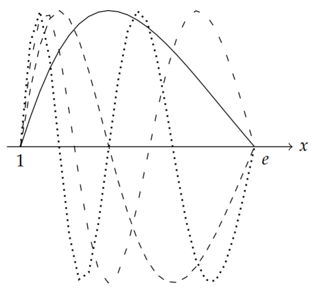
This is easily solved. The characteristic equation is

\[r^{2}+(1+\lambda)=0 .\nonumber \]

One obtains nontrivial solutions of the eigenvalue problem satisfying the boundary conditions when \(\lambda>-1\). The solutions are

\[\phi_{n}(x)=A \sin (n \pi \ln x), \quad n=1,2, \ldots\nonumber \]

where \(\lambda_{n}=n^{2} \pi^{2}-1\).

It is often useful to normalize the eigenfunctions. This means that one chooses A so that the norm of each eigenfunction is one. Thus, we have

\[\begin{align} 1 &=\int_{1}^{e} \phi_{n}(x)^{2} \sigma(x) d x\nonumber \\ &=A^{2} \int_{1}^{e} \sin (n \pi \ln x) \frac{1}{x} d x\nonumber \\ &=A^{2} \int_{0}^{1} \sin (n \pi y) d y=\frac{1}{2} A^{2} .\label{eq:4} \end{align} \]

Thus, \(A=\sqrt{2}\). Several of these eigenfunctions are show in Figure \(\PageIndex{1}\).

Figure \(\PageIndex{1}\): Plots of the first five eigenfunctions, \(y(x)=\sqrt{2} \sin (n \pi \ln x)\).

We now turn towards solving the nonhomogeneous problem, \(\mathcal{L} y=\frac{1}{x}\). We first expand the unknown solution in terms of the eigenfunctions,

\[y(x)=\sum_{n=1}^{\infty} c_{n} \sqrt{2} \sin (n \pi \ln x) .\nonumber \]

Inserting this solution into the differential equation, we have

\[\frac{1}{x}=\mathcal{L} y=-\sum_{n=1}^{\infty} c_{n} \lambda_{n} \sqrt{2} \sin (n \pi \ln x) \frac{1}{x} .\nonumber \]

Next, we make use of orthogonality. Multiplying both sides by the eigenfunction \(\phi_{m}(x)=\sqrt{2} \sin (m \pi \ln x)\) and integrating, gives

\[\lambda_{m} c_{m}=\int_{1}^{e} \sqrt{2} \sin (m \pi \ln x) \frac{1}{x} d x=\frac{\sqrt{2}}{m \pi}\left[(-1)^{m}-1\right] .\nonumber \]

Solving for \(c_{m}\), we have

\[c_{m}=\frac{\sqrt{2}}{m \pi} \frac{\left[(-1)^{m}-1\right]}{m^{2} \pi^{2}-1} .\nonumber \]

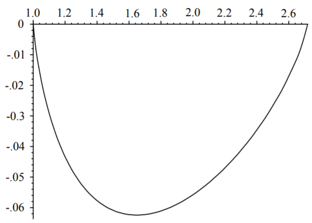
Finally, we insert these coefficients into the expansion for \(y(x)\). The solution is then

\[y(x)=\sum_{n=1}^{\infty} \frac{2}{n \pi} \frac{\left[(-1)^{n}-1\right]}{n^{2} \pi^{2}-1} \sin (n \pi \ln (x)) .\nonumber \]

We plot this solution in Figure \(\PageIndex{2}\).

Figure \(\PageIndex{2}\): Plot of the solution in Example \(\PageIndex{1}\).