6.1: Vibrations of Rectangular Membranes

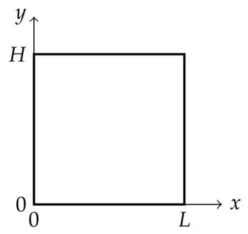
Our first example will be the study of the vibrations of a rectangular membrane. You can think of this as a drumhead with a rectangular cross section as shown in Figure \(\PageIndex{1}\). We stretch the membrane over the drumhead and fasten the material to the boundary of the rectangle. The height of the vibrating membrane is described by its height from equilibrium, \(u(x, y, t)\). This problem is a much simpler example of higher dimensional vibrations than that possessed by the oscillating electric and magnetic fields in the last chapter.

Figure \(\PageIndex{1}\): The rectangular membrane of length \(L\) and width \(H\). There are fixed boundary conditions along the edges.

Example \(\PageIndex{1}\): The Vibrating Rectangular Membrane

The problem is given by the two dimensional wave equation in Cartesian coordinates, \[u_{t t}=c^{2}\left(u_{x x}+u_{y y}\right), \quad t>0,0<x<L, 0<y<H,\label{eq:1}\] a set of boundary conditions, \[\begin{array}{ll} u(0, y, t)=0, & u(L, y, t)=0, \quad t>0, \quad 0<y<H, \\ u(x, 0, t)=0, & u(x, H, t)=0, \quad t>0, \quad 0<x<L, \end{array}\label{eq:2}\] and a pair of initial conditions (since the equation is second order in time), \[u(x, y, 0)=f(x, y), \quad u_{t}(x, y, 0)=g(x, y) .\label{eq:3}\]

The first step is to separate the variables: \(u(x, y, t)=X(x) Y(y) T(t)\). Inserting the guess, \(u(x, y, t)\) into the wave equation, we have \[X(x) Y(y) T^{\prime \prime}(t)=c^{2}\left(X^{\prime \prime}(x) Y(y) T(t)+X(x) Y^{\prime \prime}(y) T(t)\right) .\nonumber \] Dividing by both \(u(x, y, t)\) and \(c^{2}\), we obtain \[\underbrace{\frac{1}{c^{2}} \frac{T^{\prime \prime}}{T}}_{\text {unction of } t}=\underbrace{\frac{X^{\prime \prime}}{X}+\frac{Y^{\prime \prime}}{Y}}_{\text {Function of } x \text { and } y}=-\lambda .\label{eq:4}\]

We see that we have a function of \(t\) equals a function of \(x\) and \(y\). Thus, both expressions are constant. We expect oscillations in time, so we choose the constant \(\lambda\) to be positive, \(\lambda>0\). (Note: As usual, the primes mean differentiation with respect to the specific dependent variable. So, there should be no ambiguity.)

These lead to two equations: \[T^{\prime \prime}+c^{2} \lambda T=0,\label{eq:5}\] and \[\frac{X^{\prime \prime}}{X}+\frac{Y^{\prime \prime}}{Y}=-\lambda \text {. }\label{eq:6}\] We note that the spatial equation is just the separated form of Helmholtz’s equation with \(\phi(x, y)=X(x) Y(y)\).

The first equation is easily solved. We have \[T(t)=a \cos \omega t+b \sin \omega t,\label{eq:7}\] where \[\omega=c \sqrt{\lambda} \text {. }\label{eq:8}\] This is the angular frequency in terms of the separation constant, or eigenvalue. It leads to the frequency of oscillations for the various harmonics of the vibrating membrane as \[v=\frac{\omega}{2 \pi}=\frac{c}{2 \pi} \sqrt{\lambda} \text {. }\label{eq:9}\] Once we know \(\lambda\), we can compute these frequencies.

Next we solve the spatial equation. We need carry out another separation of variables. Rearranging the spatial equation, we have \[\underbrace{\frac{X^{\prime \prime}}{X}}_{\text {Function of } x}=\underbrace{-\frac{Y^{\prime \prime}}{Y}-\lambda}_{\text {Function of } y}=-\mu .\label{eq:10}\] Here we have a function of \(x\) equal to a function of \(y\). So, the two expressions are constant, which we indicate with a second separation constant, \(-\mu<0\). We pick the sign in this way because we expect oscillatory solutions for \(X(x)\). This leads to two equations: \[\begin{array}{r} X^{\prime \prime}+\mu X=0, \\ Y^{\prime \prime}+(\lambda-\mu) Y=0 . \end{array}\label{eq:11}\]

We now impose the boundary conditions. We have \(u(0, y, t)=0\) for all \(t>0\) and \(0<y<H\). This implies that \(X(0) Y(y) T(t)=0\) for all \(t\) and \(y\) in the domain. This is only true if \(X(0)=0\). Similarly, from the other boundary conditions we find that \(X(L)=0, Y(0)=0\), and \(Y(H)=0\). We note that homogeneous boundary conditions are important in carrying out this process. Nonhomogeneous boundary conditions could be imposed just like we had in Section 7.3, but we still need the solutions for homogeneous boundary conditions before tackling the more general problems.

In summary, the boundary value problems we need to solve are: \[\begin{align} X^{\prime \prime}+\mu X &=0, \quad X(0)=0, X(L)=0 .\nonumber \\ Y^{\prime \prime}+(\lambda-\mu) Y &=0, \quad Y(0)=0, Y(H)=0 .\label{eq:12} \end{align}\]

We have seen boundary value problems of these forms in Chapter ??. The solutions of the first eigenvalue problem are \[X_{n}(x)=\sin \frac{n \pi x}{L}, \quad \mu_{n}=\left(\frac{n \pi}{L}\right)^{2}, \quad n=1,2,3, \ldots\nonumber \]

The second eigenvalue problem is solved in the same manner. The differences from the first problem are that the "eigenvalue" is \(\lambda-\mu\), the independent variable is \(y\), and the interval is \([0, H]\). Thus, we can quickly write down the solutions as \[Y_{m}(y)=\sin \frac{m \pi x}{H}, \quad \lambda-\mu_{m}=\left(\frac{m \pi}{H}\right)^{2}, \quad m=1,2,3, \ldots\nonumber \]

At this point we need to be careful about the indexing of the separation constants. So far, we have seen that \(\mu\) depends on \(n\) and that the quantity \(\kappa=\lambda-\mu\) depends on \(m\). Solving for \(\lambda\), we should write \(\lambda_{n m}=\mu_{n}+\kappa_{m}\), or \[\lambda_{n m}=\left(\frac{n \pi}{L}\right)^{2}+\left(\frac{m \pi}{H}\right)^{2}, \quad n, m=1,2, \ldots .\label{eq:13}\] Since \(\omega=c \sqrt{\lambda}\), we have that the discrete frequencies of the harmonics are given by \[\omega_{n m}=c \sqrt{\left(\frac{n \pi}{L}\right)^{2}+\left(\frac{m \pi}{H}\right)^{2}}, \quad n, m=1,2, \ldots\label{eq:14}\]

Note

The harmonics for the vibrating rectangular membrane are given by \[v_{n m}=\frac{c}{2} \sqrt{\left(\frac{n}{L}\right)^{2}+\left(\frac{m}{H}\right)^{2}}\nonumber \] for \(n, m=1,2, \ldots\)

We have successfully carried out the separation of variables for the wave equation for the vibrating rectangular membrane. The product solutions can be written as \[u_{n m}=\left(a \cos \omega_{n m} t+b \sin \omega_{n m} t\right) \sin \frac{n \pi x}{L} \sin \frac{m \pi y}{H}\label{eq:15}\] and the most general solution is written as a linear combination of the product solutions, \[u(x, y, t)=\sum_{n, m}\left(a_{n m} \cos \omega_{n m} t+b_{n m} \sin \omega_{n m} t\right) \sin \frac{n \pi x}{L} \sin \frac{m \pi y}{H} .\nonumber \] However, before we carry the general solution any further, we will first concentrate on the two dimensional harmonics of this membrane.

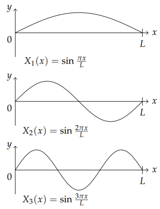
For the vibrating string the \(n\)th harmonic corresponds to the function \(\sin \frac{n \pi x}{L}\) and several are shown in Figure \(\PageIndex{2}\). The various harmonics correspond to the pure tones supported by the string. These then lead to the corresponding frequencies that one would hear. The actual shapes of the harmonics are sketched by locating the nodes, or places on the string that do not move.

Figure \(\PageIndex{2}\): The first harmonics of the vibrating string

In the same way, we can explore the shapes of the harmonics of the vibrating membrane. These are given by the spacial functions \[\phi_{n m}(x, y)=\sin \frac{n \pi x}{L} \sin \frac{m \pi y}{H} .\label{eq:16}\] Instead of nodes, we will look for the nodal curves, or nodal lines. These are the points \((x, y)\) at which \(\phi_{n m}(x, y)=0\). Of course, these depend on the indices, \(n\) and \(m\).

For example, when \(n=1\) and \(m=1\), we have \[\sin \frac{\pi x}{L} \sin \frac{\pi y}{H}=0 .\nonumber \]

Figure \(\PageIndex{3}\): The first few modes of the vibrating rectangular membrane. The dashed lines show the nodal lines indicating the points that do not move for the particular mode. Compare these the nodal lines to the \({ }_{3} \mathrm{D}\) view in Figure \(\PageIndex{1}\).

These are zero when either \[\sin \frac{\pi x}{L}=0, \text { or } \sin \frac{\pi y}{H}=0 .\nonumber \] Of course, this can only happen for \(x=0, L\) and \(y=0, H\). Thus, there are no interior nodal lines.

When \(n=2\) and \(m=1\), we have \(y=0, H\) and \[\sin \frac{2 \pi x}{L}=0\nonumber \] or, \(x=0, \frac{L}{2}, L\). Thus, there is one interior nodal line at \(x=\frac{L}{2}\). These points stay fixed during the oscillation and all other points oscillate on either side of this line. A similar solution shape results for the \((1,2)\)-mode; i.e., \(n=1\) and \(m=2\).

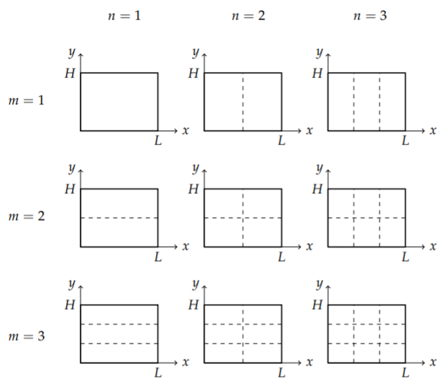
In Figure \(\PageIndex{3}\) we show the nodal lines for several modes for \(n, m=1,2,3\) with different columns corresponding to different \(n\)-values while the rows are labeled with different \(m\)-values. The blocked regions appear to vibrate independently. A better view is the three dimensional view depicted in Figure \(\PageIndex{1}\). The frequencies of vibration are easily computed using the formula for \(\omega_{n m}\).

For completeness, we now return to the general solution and apply the initial conditions. The general solution is given by a linear superposition of the product solutions. There are two indices to sum over. Thus, the general solution is \[u(x, y, t)=\sum_{n=1}^{\infty} \sum_{m=1}^{\infty}\left(a_{n m} \cos \omega_{n m} t+b_{n m} \sin \omega_{n m} t\right) \sin \frac{n \pi x}{L} \sin \frac{m \pi y}{H}\label{eq:17}\]

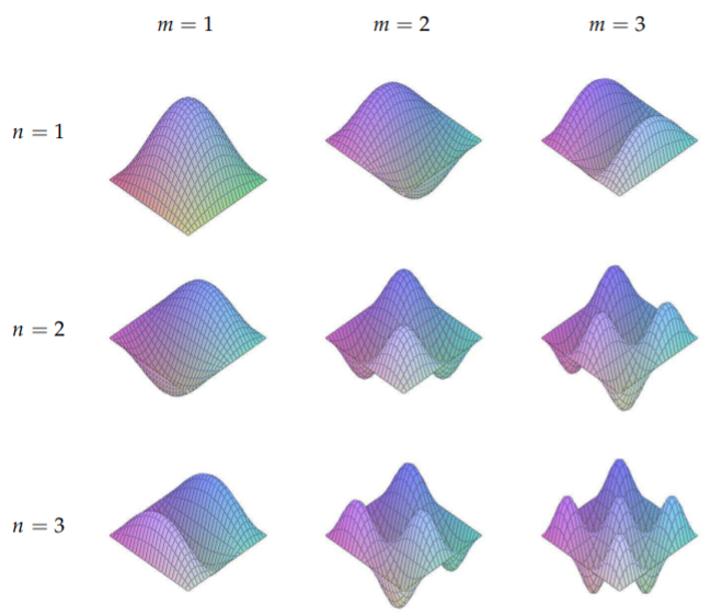
Table \(\PageIndex{1}\): A three dimensional view of the vibrating rectangular membrane for the lowest modes. Compare these images with the nodal lines in Figure \(\PageIndex{3}\).

where \[\omega_{n m}=c \sqrt{\left(\frac{n \pi}{L}\right)^{2}+\left(\frac{m \pi}{H}\right)^{2}} .\label{eq:18}\]

The first initial condition is \(u(x, y, 0)=f(x, y)\). Setting \(t=0\) in the general solution, we obtain \[f(x, y)=\sum_{n=1}^{\infty} \sum_{m=1}^{\infty} a_{n m} \sin \frac{n \pi x}{L} \sin \frac{m \pi y}{H} .\label{eq:19}\] This is a double Fourier sine series. The goal is to find the unknown coefficients \(a_{n m}\).

The coefficients \(a_{n m}\) can be found knowing what we already know about Fourier sine series. We can write the initial condition as the single sum \[f(x, y)=\sum_{n=1}^{\infty} A_{n}(y) \sin \frac{n \pi x}{L},\label{eq:20}\] where \[A_{n}(y)=\sum_{m=1}^{\infty} a_{n m} \sin \frac{m \pi y}{H} .\label{eq:21}\]

These are two Fourier sine series. Recalling from Chapter ?? that the coefficients of Fourier sine series can be computed as integrals, we have \[\begin{align} A_{n}(y) &=\frac{2}{L} \int_{0}^{L} f(x, y) \sin \frac{n \pi x}{L} d x,\nonumber \\ a_{n m} &=\frac{2}{H} \int_{0}^{H} A_{n}(y) \sin \frac{m \pi y}{H} d y .\label{eq:22} \end{align}\]

Inserting the integral for \(A_{n}(y)\) into that for \(a_{n m}\), we have an integral representation for the Fourier coefficients in the double Fourier sine series, \[a_{n m}=\frac{4}{L H} \int_{0}^{H} \int_{0}^{L} f(x, y) \sin \frac{n \pi x}{L} \sin \frac{m \pi y}{H} d x d y .\label{eq:23}\]

We can carry out the same process for satisfying the second initial condition, \(u_{t}(x, y, 0)=g(x, y)\) for the initial velocity of each point. Inserting the general solution into this initial condition, we obtain \[g(x, y)=\sum_{n=1}^{\infty} \sum_{m=1}^{\infty} b_{n m} \omega_{n m} \sin \frac{n \pi x}{L} \sin \frac{m \pi y}{H} .\label{eq:24}\] Again, we have a double Fourier sine series. But, now we can quickly determine the Fourier coefficients using the above expression for \(a_{n m}\) to find that \[b_{n m}=\frac{4}{\omega_{n m} L H} \int_{0}^{H} \int_{0}^{L} g(x, y) \sin \frac{n \pi x}{L} \sin \frac{m \pi y}{H} d x d y .\label{eq:25}\]

This completes the full solution of the vibrating rectangular membrane problem. Namely, we have obtained the solution \[u(x, y, t)=\sum_{n=1}^{\infty} \sum_{m=1}^{\infty}\left(a_{n m} \cos \omega_{n m} t+b_{n m} \sin \omega_{n m} t\right) \sin \frac{n \pi x}{L} \sin \frac{m \pi y}{H}\label{eq:26}\] where \[a_{n m}=\frac{4}{L H} \int_{0}^{H} \int_{0}^{L} f(x, y) \sin \frac{n \pi x}{L} \sin \frac{m \pi y}{H} d x d y,\label{eq:27}\] \[ b_{n m}=\frac{4}{\omega_{n m} L H} \int_{0}^{H} \int_{0}^{L} g(x, y) \sin \frac{n \pi x}{L} \sin \frac{m \pi y}{H} d x d y, \label{eq:28}\] and the angular frequencies are given by \[\omega_{n m}=c \sqrt{\left(\frac{n \pi}{L}\right)^{2}+\left(\frac{m \pi}{H}\right)^{2}} .\label{eq:29}\]