6.3: Laplace’s Equation in 2D

Another of the generic partial differential equations is Laplace’s equation, \(\nabla^{2} u=0\). This equation first appeared in the chapter on complex variables when we discussed harmonic functions. Another example is the electric potential for electrostatics. As we described Chapter ??, for static electromagnetic fields, \[\nabla \cdot \mathbf{E}=\rho / \epsilon_{0}, \quad \mathbf{E}=\nabla \phi .\nonumber \] In regions devoid of charge, these equations yield the Laplace equation \(\nabla^{2} \phi=0\).

Another example comes from studying temperature distributions. Consider a thin rectangular plate with the boundaries set at fixed temperatures. Temperature changes of the plate are governed by the heat equation. The solution of the heat equation subject to these boundary conditions is time dependent. In fact, after a long period of time the plate will reach thermal equilibrium. If the boundary temperature is zero, then the plate temperature decays to zero across the plate. However, if the boundaries are maintained at a fixed nonzero temperature, which means energy is being put into the system to maintain the boundary conditions, the internal temperature may reach a nonzero equilibrium temperature. Reaching thermal equilibrium means that asymptotically in time the solution becomes time independent. Thus, the equilibrium state is a solution of the time independent heat equation, which is another Laplace equation, \(\nabla^{2} u=0\).

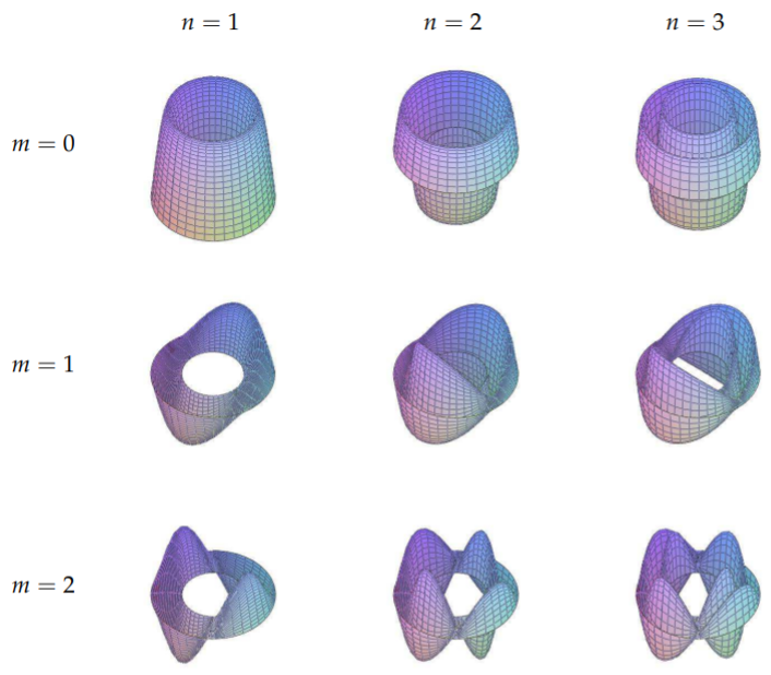
Table \(\PageIndex{1}\): A three dimensional view of the vibrating annular membrane for the lowest modes.

Note

Thermodynamic equilibrium, \(\nabla^{2} u=0\).

Note

Incompressible, irrotational fluid flow, \(\nabla^{2} \phi=0\), for velocity \(\mathbf{v}=\nabla \phi .\)

As another example we could look at fluid flow. For an incompressible flow, \(\nabla \cdot \mathbf{v}=0\). If the flow is irrotational, then \(\nabla \times \mathbf{v}=0\). We can introduce a velocity potential, \(\mathbf{v}=\nabla \phi\). Thus, \(\nabla \times \mathbf{v}\) vanishes by a vector identity and \(\nabla \cdot \mathbf{v}=0\) implies \(\nabla^{2} \phi=0\). So, once again we obtain Laplace’s equation.

In this section we will look at examples of Laplace’s equation in two dimensions. The solutions in these examples could be examples from any of the application in the above physical situations and the solutions can be applied appropriately.

Example \(\PageIndex{1}\): Equilibruim Temperature Distribution for a Rectangular Plate

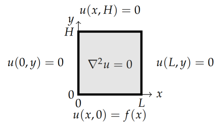
Let’s consider Laplace’s equation in Cartesian coordinates, \[u_{x x}+u_{y y}=0, \quad 0<x<L, \quad 0<y<H\nonumber \] with the boundary conditions \[u(0, y)=0, \quad u(L, y)=0, \quad u(x, 0)=f(x), \quad u(x, H)=0 .\nonumber \] The boundary conditions are shown in Figure \(\PageIndex{1}\).

Figure \(\PageIndex{1}\): In this figure we show the domain and boundary conditions for the example of determining the equilibrium temperature for a rectangular plate.

Solution

As with the heat and wave equations, we can solve this problem using the method of separation of variables. Let \(u(x, y)=X(x) Y(y)\). Then, Laplace’s equation becomes \[X^{\prime \prime} Y+X Y^{\prime \prime}=0\nonumber \] and we can separate the \(x\) and \(y\) dependent functions and introduce a separation constant, \(\lambda\), \[\frac{X^{\prime \prime}}{X}=-\frac{Y^{\prime \prime}}{Y}=-\lambda \text {. }\nonumber \] Thus, we are led to two differential equations, \[\begin{align} &X^{\prime \prime}+\lambda X=0\nonumber \\ &Y^{\prime \prime}-\lambda Y=0\label{eq:1} \end{align}\]

From the boundary condition \(u(0, y)=0, u(L, y)=0\), we have \(X(0)=\) \(0, X(L)=0 .\) So, we have the usual eigenvalue problem for \(X(x)\), \[X^{\prime \prime}+\lambda X=0, \quad X(0)=0, X(L)=0 .\nonumber \] The solutions to this problem are given by \[X_{n}(x)=\sin \frac{n \pi x}{L}, \quad \lambda_{n}=\left(\frac{n \pi}{L}\right)^{2}, \quad n=1,2, \ldots\nonumber \]

The general solution of the equation for \(Y(y)\) is given by \[Y(y)=c_{1} e^{\sqrt{\lambda} y}+c_{2} e^{-\sqrt{\lambda} y}\nonumber \] The boundary condition \(u(x, H)=0\) implies \(Y(H)=0 .\) So, we have \[c_{1} e^{\sqrt{\lambda H}}+c_{2} e^{-\sqrt{\lambda H}}=0 .\nonumber \] Thus, \[c_{2}=-c_{1} e^{2 \sqrt{\lambda} H} .\nonumber \] Inserting this result into the expression for \(Y(y)\), we have \[\begin{align} Y(y) &=c_{1} e^{\sqrt{\lambda} y}-c_{1} e^{2 \sqrt{\lambda} H} e^{-\sqrt{\lambda} y}\nonumber \\ &=c_{1} e^{\sqrt{\lambda} H}\left(e^{-\sqrt{\lambda} H} e^{\sqrt{\lambda} y}-e^{\sqrt{\lambda} H} e^{-\sqrt{\lambda} y}\right)\nonumber \\ &=c_{1} e^{\sqrt{\lambda} H}\left(e^{-\sqrt{\lambda}(H-y)}-e^{\sqrt{\lambda}(H-y)}\right)\nonumber \\ &=-2 c_{1} e^{\sqrt{\lambda} H} \sinh \sqrt{\lambda}(H-y)\label{eq:2} \end{align}\]

Note

Having carried out this computation, we can now see that it would be better to guess this form in the future. So, for \(Y(H)=0\), one would guess a solution \(Y(y)=\sinh \sqrt{\lambda}(H-y)\) For \(Y(0)=0\), one would guess a solution \(Y(y)=\sinh \sqrt{\lambda} y\). Similarly, if \(Y^{\prime}(H)=0\), one would guess a solution \(Y(y)=\cosh \sqrt{\lambda}(H-y)\)

Since we already know the values of the eigenvalues \(\lambda_{n}\) from the eigenvalue problem for \(X(x)\), we have that the \(y\)-dependence is given by \[Y_{n}(y)=\sinh \frac{n \pi(H-y)}{L} .\nonumber \] So, the product solutions are given by \[u_{n}(x, y)=\sin \frac{n \pi x}{L} \sinh \frac{n \pi(H-y)}{L}, \quad n=1,2, \ldots\nonumber \] These solutions satisfy Laplace’s equation and the three homogeneous boundary conditions and in the problem.

The remaining boundary condition, \(u(x, 0)=f(x)\), still needs to be satisfied. Inserting \(y=0\) in the product solutions does not satisfy the boundary condition unless \(f(x)\) is proportional to one of the eigenfunctions \(X_{n}(x)\). So, we first write down the general solution as a linear combination of the product solutions, \[u(x, y)=\sum_{n=1}^{\infty} a_{n} \sin \frac{n \pi x}{L} \sinh \frac{n \pi(H-y)}{L} .\label{eq:3}\]

Now we apply the boundary condition, \(u(x, 0)=f(x)\), to find that \[f(x)=\sum_{n=1}^{\infty} a_{n} \sinh \frac{n \pi H}{L} \sin \frac{n \pi x}{L} .\label{eq:4}\] Defining \(b_{n}=a_{n} \sinh \frac{n \pi H}{L}\), this becomes \[f(x)=\sum_{n=1}^{\infty} b_{n} \sin \frac{n \pi x}{L} .\label{eq:5}\] We see that the determination of the unknown coefficients, \(b_{n}\), is simply done by recognizing that this is a Fourier sine series. The Fourier coefficients are easily found as \[b_{n}=\frac{2}{L} \int_{0}^{L} f(x) \sin \frac{n \pi x}{L} d x .\label{eq:6}\]

Since \(a_{n}=b_{n} / \sinh \frac{n \pi H}{L}\), we can finish solving the problem. The solution is \[u(x,y)=\sum\limits_{n=1}^\infty a_n\sin\frac{n\pi x}{L}\sinh\frac{n\pi (H-y)}{L},\label{eq:7}\] where \[a_{n}=\frac{2}{L \sinh \frac{n \pi H}{L}} \int_{0}^{L} f(x) \sin \frac{n \pi x}{L} d x\label{eq:8}\]

Example \(\PageIndex{2}\): Equilibrium Temperature Distribution for a Rectangular Plate for General Boundary Conditions

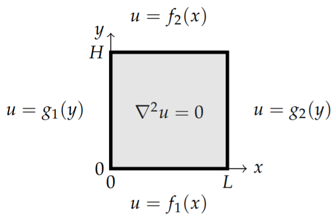
A more general problem is to seek solutions to Laplace’s equation in Cartesian coordinates, \[u_{x x}+u_{y y}=0, \quad 0<x<L, 0<y<H\nonumber \] with non-zero boundary conditions on more than one side of the domain, \[\begin{array}{ll} u(0, y)=g_{1}(y), \quad u(L, y)=g_{2}(y), \quad 0<y<H, \\ u(x, 0)=f_{1}(x), \quad u(x, H)=f_{2}(x), \quad 0<x<L . \end{array}\nonumber \] These boundary conditions are shown in Figure \(\PageIndex{2}\).

Figure \(\PageIndex{2}\): In this figure we show the domain and general boundary conditions for the example of determining the equilibrium temperature distribution for a rectangular plate.

Solution

The problem with this example is that none of the boundary conditions are homogeneous. This means that the corresponding eigenvalue problems will not have the homogeneous boundary conditions which Sturm-Liouville theory in Section 4 needs. However, we can express this problem in terms of four different problems with nonhomogeneous boundary conditions on only one side of the rectangle.

Figure \(\PageIndex{3}\): The general boundary value problem for a rectangular plate can be written as the sum of these four separate problems.

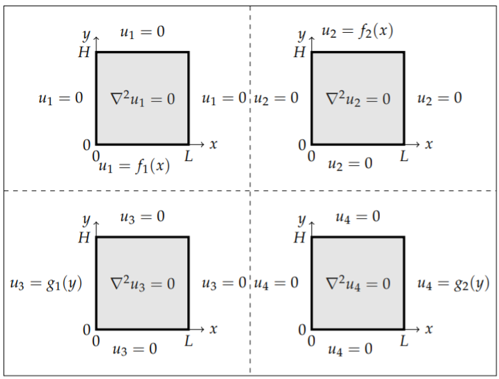
In Figure \(\PageIndex{3}\) we show how the problem can be broken up into four separate problems for functions \(u_{i}(x, y), i=1, \ldots, 4\). Since the boundary conditions and Laplace’s equation are linear, the solution to the general problem is simply the sum of the solutions to these four problems, \[u(x, y)=u_{1}(x, y)+u_{2}(x, y)+u_{3}(x, y)+u_{4}(x, y) .\nonumber \] Then, this solution satisfies Laplace’s equation, \[\nabla^{2} u(x, y)=\nabla^{2} u_{1}(x, y)+\nabla^{2} u_{2}(x, y)+\nabla^{2} u_{3}(x, y)+\nabla^{2} u_{4}(x, y)=0,\nonumber \] and the boundary conditions. For example, using the boundary conditions defined in Figure \(\PageIndex{3}\), we have for \(y=0\), \[u(x, 0)=u_{1}(x, 0)+u_{2}(x, 0)+u_{3}(x, 0)+u_{4}(x, 0)=f_{1}(x) .\nonumber \] The other boundary conditions can also be shown to hold.

We can solve each of the problems in Figure \(\PageIndex{3}\) quickly based on the solution we obtained in the last example. The solution for \(u_{1}(x, y)\), which satisfies the boundary conditions \[\begin{gathered} u_{1}(0, y)=0, \quad u_{1}(L, y)=0, \quad 0<y<H, \\ u_{1}(x, 0)=f_{1}(x), \quad u_{1}(x, H)=0, \quad 0<x<L, \end{gathered}\nonumber \] is the easiest to write down. It is given by \[u_{1}(x, y)=\sum_{n=1}^{\infty} a_{n} \sin \frac{n \pi x}{L} \sinh \frac{n \pi(H-y)}{L} .\label{eq:9}\] where \[a_{n}=\frac{2}{L \sinh \frac{n \pi H}{L}} \int_{0}^{L} f_{1}(x) \sin \frac{n \pi x}{L} d x\label{eq:10}\]

For the boundary conditions \[\begin{gathered} u_{2}(0, y)=0, \quad u_{2}(L, y)=0, \quad 0<y<H, \\ u_{2}(x, 0)=0, \quad u_{2}(x, H)=f_{2}(x), \quad 0<x<L . \end{gathered}\nonumber \] the boundary conditions for \(X(x)\) are \(X(0)=0\) and \(X(L)=0\). So, we get the same form for the eigenvalues and eigenfunctions as before: \[X_{n}(x)=\sin \frac{n \pi x}{L}, \quad \lambda_{n}=\left(\frac{n \pi}{L}\right)^{2}, n=1,2, \ldots .\nonumber \]

The remaining homogeneous boundary condition is now \(Y(0)=0\). Recalling that the equation satisfied by \(Y(y)\) is \[Y^{\prime \prime}-\lambda Y=0,\nonumber \] we can write the general solution as \[Y(y)=c_{1} \cosh \sqrt{\lambda} y+c_{2} \sinh \sqrt{\lambda} y .\nonumber \]

Requiring \(Y(0)=0\), we have \(c_{1}=0\), or \[Y(y)=c_{2} \sinh \sqrt{\lambda} y .\nonumber \] Then, the general solution is \[u_{2}(x, y)=\sum_{n=1}^{\infty} b_{n} \sin \frac{n \pi x}{L} \sinh \frac{n \pi y}{L} .\label{eq:11}\]

We now force the nonhomogeneous boundary condition, \(u_{2}(x, H)=f_{2}(x)\), \[f_{2}(x)=\sum_{n=1}^{\infty} b_{n} \sin \frac{n \pi x}{L} \sinh \frac{n \pi H}{L} .\label{eq:12}\] Once again we have a Fourier sine series. The Fourier coefficients are given by \[b_{n}=\frac{2}{L \sinh \frac{n \pi H}{L}} \int_{0}^{L} f_{2}(x) \sin \frac{n \pi x}{L} d x .\label{eq:13}\]

Next we turn to the problem with the boundary conditions \[\begin{gathered} u_{3}(0, y)=g_{1}(y), \quad u_{3}(L, y)=0, \quad 0<y<H, \\ u_{3}(x, 0)=0, \quad u_{3}(x, H)=0, \quad 0<x<L . \end{gathered}\nonumber \] In this case the pair of homogeneous boundary conditions \(u_{3}(x, 0)=0, \quad u_{3}(x, H)=\) 0 lead to solutions \[Y_{n}(y)=\sin \frac{n \pi y}{H}, \quad \lambda_{n}=-\left(\frac{n \pi}{H}\right)^{2}, \quad n=1,2 \ldots .\nonumber \] The condition \(u_{3}(L, 0)=0\) gives \(X(x)=\sinh \frac{n \pi(L-x)}{H}\).

The general solution satisfying the homogeneous conditions is \[u_{3}(x, y)=\sum_{n=1}^{\infty} c_{n} \sin \frac{n \pi y}{H} \sinh \frac{n \pi(L-x)}{H} .\label{eq:14}\] Applying the nonhomogeneous boundary condition, \(u_{3}(0, y)=g_{1}(y)\), we obtain the Fourier sine series \[g_{1}(y)=\sum_{n=1}^{\infty} c_{n} \sin \frac{n \pi y}{H} \sinh \frac{n \pi L}{H} .\label{eq:15}\] The Fourier coefficients are found as \[c_{n}=\frac{2}{H \sinh \frac{n \pi L}{H}} \int_{0}^{H} g_{1}(y) \sin \frac{n \pi y}{H} d y .\label{eq:16}\]

Finally, we can find the solution \[\begin{gathered} u_{4}(0, y)=0, \quad u_{4}(L, y)=g_{2}(y), \quad 0<y<H, \\ u_{4}(x, 0)=0, \quad u_{4}(x, H)=0, \quad 0<x<L . \end{gathered}\nonumber \] Following the above analysis, we find the general solution \[u_{4}(x, y)=\sum_{n=1}^{\infty} d_{n} \sin \frac{n \pi y}{H} \sinh \frac{n \pi x}{H} .\label{eq:17}\] The nonhomogeneous boundary condition, \(u(L, y)=g_{2}(y)\), is satisfied if \[g_{2}(y)=\sum_{n=1}^{\infty} d_{n} \sin \frac{n \pi y}{H} \sinh \frac{n \pi L}{H} .\label{eq:18}\] The Fourier coefficients, \(d_{n}\), are given by \[d_{n}=\frac{2}{H \sinh \frac{n \pi L}{H}} \int_{0}^{H} g_{1}(y) \sin \frac{n \pi y}{H} d y .\label{eq:19}\]

The solution to the general problem is given by the sum of these four solutions. \[\begin{align} u(x, y)=& \sum_{n=1}^{\infty}\left[\left(a_{n} \sinh \frac{n \pi(H-y)}{L}+b_{n} \sinh \frac{n \pi y}{L}\right) \sin \frac{n \pi x}{L}\right.\nonumber \\ &\left.+\left(c_{n} \sinh \frac{n \pi(L-x)}{H}+d_{n} \sinh \frac{n \pi x}{H}\right) \sin \frac{n \pi y}{H}\right],\label{eq:20} \end{align}\] where the coefficients are given by the above Fourier integrals.

Example \(\PageIndex{3}\): Laplace's Equation on a Disk

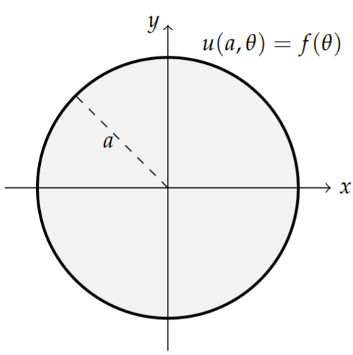
We now turn to solving Laplace’s equation on a disk of radius a as shown in Figure \(\PageIndex{4}\). Laplace’s equation in polar coordinates is given by \[\frac{1}{r} \frac{\partial}{\partial r}\left(r \frac{\partial u}{\partial r}\right)+\frac{1}{r^{2}} \frac{\partial^{2} u}{\partial \theta^{2}}=0, \quad 0<r<a, \quad-\pi<\theta<\pi .\label{eq:21}\] The boundary conditions are given as \[u(a, \theta)=f(\theta), \quad-\pi<\theta<\pi,\label{eq:22}\] plus periodic boundary conditions in \(\theta\).

Figure \(\PageIndex{4}\): The disk of radius \(a\) with or boundary condition along the edge at \(r=a\).

Solution

Separation of variable proceeds as usual. Let \(u(r, \theta)=R(r) \Theta(\theta)\). Then \[\frac{1}{r} \frac{\partial}{\partial r}\left(r \frac{\partial(R \Theta)}{\partial r}\right)+\frac{1}{r^{2}} \frac{\partial^{2}(R \Theta)}{\partial \theta^{2}}=0,\label{eq:23}\] or \[\Theta \frac{1}{r}\left(r R^{\prime}\right)^{\prime}+\frac{1}{r^{2}} R \Theta^{\prime \prime}=0 .\label{eq:24}\] Diving by \(u(r, \theta)=R(r) \Theta(\theta)\), multiplying by \(r^{2}\), and rearranging, we have \[\frac{r}{R}\left(r R^{\prime}\right)^{\prime}=-\frac{\Theta^{\prime \prime}}{\Theta}=\lambda .\label{eq:25}\]

Since this equation gives a function of \(r\) equal to a function of \(\theta\), we set the equation equal to a constant. Thus, we have obtained two differential equations, which can be written as \[\begin{align} r\left(r R^{\prime}\right)^{\prime}-\lambda R &=0\label{eq:26} \\ \Theta^{\prime \prime}+\lambda \Theta &=0\label{eq:27} \end{align}\]

We can solve the second equation subject to the periodic boundary conditions in the \(\theta\) variable. The reader should be able to confirm that \[\Theta(\theta)=a_{n} \cos n \theta+b_{n} \sin n \theta, \quad \lambda=n^{2}, n=0,1,2, \ldots\nonumber \] is the solution. Note that the \(n=0\) case just leads to a constant solution.

Inserting \(\lambda=n^{2}\) into the radial equation, we find \[r^{2} R^{\prime \prime}+r R^{\prime}-n^{2} R=0 .\nonumber \] This is a Cauchy-Euler type of ordinary differential equation. Recall that we solve such equations by guessing a solution of the form \(R(r)=r^{m}\). This leads to the characteristic equation \(m^{2}-n^{2}=0\). Therefore, \(m=\pm n\). So, \[R(r)=c_{1} r^{n}+c_{2} r^{-n} .\nonumber \] Since we expect finite solutions at the origin, \(r=0\), we can set (. Thus, the general solution is \[u(r, \theta)=\frac{a_{0}}{2}+\sum_{n=1}^{\infty}\left(a_{n} \cos n \theta+b_{n} \sin n \theta\right) r^{n} .\label{eq:28}\] Note that we have taken the constant term out of the sum and put it into a familiar form.

Now we can impose the remaining boundary condition, \(u(a, \theta)=f(\theta)\), or \[f(\theta)=\frac{a_{0}}{2}+\sum_{n=1}^{\infty}\left(a_{n} \cos n \theta+b_{n} \sin n \theta\right) a^{n} .\label{eq:29}\] This is a Fourier trigonometric series. The Fourier coefficients can be determined using the results from Chapter 4 : \[\begin{align} &a_{n}=\frac{1}{\pi a^{n}} \int_{-\pi}^{\pi} f(\theta) \cos n \theta d \theta, \quad n=0,1, \ldots,\label{eq:30} \\ &b_{n}=\frac{1}{\pi a^{n}} \int_{-\pi}^{\pi} f(\theta) \sin n \theta d \theta \quad n=1,2 \ldots .\label{eq:31} \end{align}\]

Poisson Integral Formula

We can put the solution from the last example in a more compact form by inserting the Fourier coefficients into the general solution. Doing this, we have \[\begin{align} u(r, \theta)=& \frac{a_{0}}{2}+\sum_{n=1}^{\infty}\left(a_{n} \cos n \theta+b_{n} \sin n \theta\right) r^{n}\nonumber \\ =& \frac{1}{2 \pi} \int_{-\pi}^{\pi} f(\phi) d \phi\nonumber \\ &+\frac{1}{\pi} \int_{-\pi}^{\pi} \sum_{n=1}^{\infty}[\cos n \phi \cos n \theta+\sin n \phi \sin n \theta]\left(\frac{r}{a}\right)^{n} f(\phi) d \phi\nonumber \\ =& \frac{1}{\pi} \int_{-\pi}^{\pi}\left[\frac{1}{2}+\sum_{n=1}^{\infty} \cos n(\theta-\phi)\left(\frac{r}{a}\right)^{n}\right] f(\phi) d \phi .\label{eq:32} \end{align}\]

The term in the brackets can be summed. We note that \[\begin{align} \cos n(\theta-\phi)\left(\frac{r}{a}\right)^{n} &=\operatorname{Re}\left(e^{i n(\theta-\phi)}\left(\frac{r}{a}\right)^{n}\right)\nonumber \\ &=\operatorname{Re}\left(\frac{r}{a} e^{i(\theta-\phi)}\right)^{n} .\label{eq:33} \end{align}\] Therefore, \[\sum_{n=1}^{\infty} \cos n(\theta-\phi)\left(\frac{r}{a}\right)^{n}=\operatorname{Re}\left(\sum_{n=1}^{\infty}\left(\frac{r}{a} e^{i(\theta-\phi)}\right)^{n}\right) .\nonumber \] The right hand side of this equation is a geometric series with common ratio of \(\frac{r}{a} e^{i(\theta-\phi)}\), which is also the first term of the series. Since \(\left|\frac{r}{a} e^{i(\theta-\phi)}\right|=\frac{r}{a}<1\), the series converges. Summing the series, we obtain \[\begin{align} \sum_{n=1}^{\infty}\left(\frac{r}{a} e^{i(\theta-\phi)}\right)^{n} &=\frac{\frac{r}{a} e^{i(\theta-\phi)}}{1-\frac{r}{a} e^{i(\theta-\phi)}}\nonumber \\ &=\frac{r e^{i(\theta-\phi)}}{a-r e^{i(\theta-\phi)}}\label{eq:34} \end{align}\]

We need to rewrite this result so that we can easily take the real part. Thus, we multiply and divide by the complex conjugate of the denominator to obtain \[\begin{align} \sum_{n=1}^{\infty}\left(\frac{r}{a} e^{i(\theta-\phi)}\right)^{n} &=\frac{r e^{i(\theta-\phi)}}{a-r e^{i(\theta-\phi)}} \frac{a-r e^{-i(\theta-\phi)}}{a-r e^{-i(\theta-\phi)}}\nonumber \\ &=\frac{a r e^{-i(\theta-\phi)}-r^{2}}{a^{2}+r^{2}-2 a r \cos (\theta-\phi)} .\label{eq:35} \end{align}\] The real part of the sum is given as \[\operatorname{Re}\left(\sum_{n=1}^{\infty}\left(\frac{r}{a} e^{i(\theta-\phi)}\right)^{n}\right)=\frac{a r \cos (\theta-\phi)-r^{2}}{a^{2}+r^{2}-2 a r \cos (\theta-\phi)} .\nonumber\]

Therefore, the factor in the brackets under the integral in Equation \(\eqref{eq:32}\) is \[\begin{align} \frac{1}{2}+\sum_{n=1}^{\infty} \cos n(\theta-\phi)\left(\frac{r}{a}\right)^{n} &=\frac{1}{2}+\frac{\operatorname{arcos}(\theta-\phi)-r^{2}}{a^{2}+r^{2}-2 \operatorname{arcos}(\theta-\phi)}\nonumber \\ &=\frac{a^{2}-r^{2}}{2\left(a^{2}+r^{2}-2 \operatorname{arcos}(\theta-\phi)\right)}\label{eq:36} \end{align}\]

Thus, we have shown that the solution of Laplace’s equation on a disk of radius \(a\) with boundary condition \(u(a, \theta)=f(\theta)\) can be written in the closed form \[u(r, \theta)=\frac{1}{2 \pi} \int_{-\pi}^{\pi} \frac{a^{2}-r^{2}}{a^{2}+r^{2}-2 a r \cos (\theta-\phi)} f(\phi) d \phi .\label{eq:37}\] This result is called the Poisson Integral Formula and \[K(\theta, \phi)=\frac{a^{2}-r^{2}}{a^{2}+r^{2}-2 a r \cos (\theta-\phi)}\nonumber \] is called the Poisson kernel.

Example \(\PageIndex{4}\)

Evaluate the solution \(\eqref{eq:37}\) at the center of the disk.

Solution

We insert \(r=0\) into the solution \(\eqref{eq:37}\) to obtain \[u(0, \theta)=\frac{1}{2 \pi} \int_{-\pi}^{\pi} f(\phi) d \phi .\nonumber \] Recalling that the average of a function \(g(x)\) on \([a, b]\) is given by \[g_{\text {ave }}=\frac{1}{b-a} \int_{a}^{b} g(x) d x,\nonumber \] we see that the value of the solution \(u\) at the center of the disk is the average of the boundary values. This is sometimes referred to as the mean value theorem.