7.2: Boundary Value Green’s Functions

We solved nonhomogeneous initial value problems in Section 7.1 using a Green’s function. In this section we will extend this method to the solution of nonhomogeneous boundary value problems using a boundary value Green’s function. Recall that the goal is to solve the nonhomogeneous differential equation \[L[y]=f, \quad a \leq x \leq b,\nonumber \] where \(L\) is a differential operator and \(y(x)\) satisfies boundary conditions at \(x=a\) and \(x=b\).. The solution is formally given by \[y=L^{-1}[f] \text {. }\nonumber \] The inverse of a differential operator is an integral operator, which we seek to write in the form \[y(x)=\int_{a}^{b} G(x, \xi) f(\xi) d \xi .\nonumber \] The function \(G(x, \xi)\) is referred to as the kernel of the integral operator and is called the Green’s function.

We will consider boundary value problems in Sturm-Liouville form, \[\frac{d}{d x}\left(p(x) \frac{d y(x)}{d x}\right)+q(x) y(x)=f(x), \quad a<x<b \text {, }\label{eq:1}\] with fixed values of \(y(x)\) at the boundary, \(y(a)=0\) and \(y(b)=0\). However, the general theory works for other forms of homogeneous boundary conditions.

We seek the Green’s function by first solving the nonhomogeneous differential equation using the Method of Variation of Parameters. Recall this method from Section B.3.3. We assume a particular solution of the form \[y_{p}(x)=c_{1}(x) y_{1}(x)+c_{2}(x) y_{2}(x),\nonumber \] which is formed from two linearly independent solution of the homogeneous problem, \(y_{i}(x), i=1,2\). We had found that the coefficient functions satisfy the equations \[\begin{align} c_{1}^{\prime}(x) y_{1}(x)+c_{2}^{\prime}(x) y_{2}(x) &=0\nonumber \\ c_{1}^{\prime}(x) y_{1}^{\prime}(x)+c_{2}^{\prime}(x) y_{2}^{\prime}(x) &=\frac{f(x)}{p(x)} .\label{eq:2} \end{align}\]

Solving this system, we obtain \[\begin{aligned} &c_{1}^{\prime}(x)=-\frac{f y_{2}}{p W\left(y_{1}, y_{2}\right)}, \\ &c_{1}^{\prime}(x)=\frac{f y_{1}}{p W\left(y_{1}, y_{2}\right)}, \end{aligned}\] where \(W\left(y_{1}, y_{2}\right)=y_{1} y_{2}^{\prime}-y_{1}^{\prime} y_{2}\) is the Wronskian. Integrating these forms and inserting the results back into the particular solution, we find \[y(x)=y_{2}(x) \int_{x_{1}}^{x} \frac{f(\xi) y_{1}(\xi)}{p(\xi) W(\xi)} d \xi-y_{1}(x) \int_{x_{0}}^{x} \frac{f(\xi) y_{2}(\xi)}{p(\xi) W(\xi)} d \xi,\nonumber \] where \(x_{0}\) and \(x_{1}\) are to be determined using the boundary values. In particular, we will seek \(x_{0}\) and \(x_{1}\) so that the solution to the boundary value problem can be written as a single integral involving a Green’s function. Note that we can absorb the solution to the homogeneous problem, \(y_{h}(x)\), into the integrals with an appropriate choice of limits on the integrals.

We now look to satisfy the conditions \(y(a)=0\) and \(y(b)=0\). First we use solutions of the homogeneous differential equation that satisfy \(y_{1}(a)=0\), \(y_{2}(b)=0\) and \(y_{1}(b) \neq 0, y_{2}(a) \neq 0\). Evaluating \(y(x)\) at \(x=0\), we have \[\begin{align} y(a) &=y_{2}(a) \int_{x_{1}}^{a} \frac{f(\xi) y_{1}(\xi)}{p(\xi) W(\xi)} d \xi-y_{1}(a) \int_{x_{0}}^{a} \frac{f(\xi) y_{2}(\xi)}{p(\xi) W(\xi)} d \xi\nonumber \\ &=y_{2}(a) \int_{x_{1}}^{a} \frac{f(\xi) y_{1}(\xi)}{p(\xi) W(\xi)} d \xi .\label{eq:3} \end{align}\] We can satisfy the condition at \(x=a\) if we choose \(x_{1}=a\).

Similarly, at \(x=b\) we find that \[\begin{align} y(b) &=y_{2}(b) \int_{x_{1}}^{b} \frac{f(\xi) y_{1}(\xi)}{p(\xi) W(\xi)} d \xi-y_{1}(b) \int_{x_{0}}^{b} \frac{f(\xi) y_{2}(\xi)}{p(\xi) W(\xi)} d \xi\nonumber \\ &=-y_{1}(b) \int_{x_{0}}^{b} \frac{f(\xi) y_{2}(\xi)}{p(\xi) W(\xi)} d \xi .\label{eq:4} \end{align}\] This expression vanishes for \(x_{0}=b\).

So, we have found that the solution takes the form \[y(x)=y_{2}(x) \int_{a}^{x} \frac{f(\xi) y_{1}(\xi)}{p(\xi) W(\xi)} d \xi-y_{1}(x) \int_{b}^{x} \frac{f(\xi) y_{2}(\xi)}{p(\xi) W(\xi)} d \xi .\label{eq:5}\]

This solution can be written in a compact form just like we had done for the initial value problem in Section 7.1. We seek a Green’s function so that the solution can be written as a single integral. We can move the functions of \(x\) under the integral. Also, since \(a<x<b\), we can flip the limits in the second integral. This gives \[y(x)=\int_{a}^{x} \frac{f(\xi) y_{1}(\xi) y_{2}(x)}{p(\xi) W(\xi)} d \tilde{\xi}+\int_{x}^{b} \frac{f(\xi) y_{1}(x) y_{2}(\xi)}{p(\xi) W(\xi)} d \xi\label{eq:6}\] This result can now be written in a compact form:

Boundary Value Green's Function

The solution of the boundary value problem \[\begin{array}{r} \frac{d}{d x}\left(p(x) \frac{d y(x)}{d x}\right)+q(x) y(x)=f(x), \quad a<x<b, \\ y(a)=0, \quad y(b)=0 . \end{array}\label{eq:7}\] takes the form \[y(x)=\int_{a}^{b} G(x, \xi) f(\xi) d \xi,\label{eq:8}\] where the Green’s function is the piecewise defined function \[G(x, \xi)= \begin{cases}\frac{y_{1}(\xi) y_{2}(x)}{p W}, & a \leq \xi \leq x, \\ \frac{y_{1}(x) y_{2}(\xi)}{p W}, & x \leq \xi \leq b,\end{cases}\label{eq:9}\] where \(y_{1}(x)\) and \(y_{2}(x)\) are solutions of the homogeneous problem satisfying \(y_{1}(a)=0, y_{2}(b)=0\) and \(y_{1}(b) \neq 0, y_{2}(a) \neq 0\).

The Green’s function satisfies several properties, which we will explore further in the next section. For example, the Green’s function satisfies the boundary conditions at \(x=a\) and \(x=b\). Thus, \[\begin{aligned} &G(a, \xi)=\frac{y_{1}(a) y_{2}(\xi)}{p W}=0, \\ &G(b, \xi)=\frac{y_{1}(\xi) y_{2}(b)}{p W}=0 . \end{aligned}\] Also, the Green’s function is symmetric in its arguments. Interchanging the arguments gives \[G(\xi, x)= \begin{cases}\frac{y_{1}(x) y_{2}(\xi)}{p W}, & a \leq x \leq \xi, \\ \frac{y_{1}(\xi) y_{2}(x)}{p W}, & \xi \leq x \leq b,\end{cases}\label{eq:10}\] But a careful look at the original form shows that \[G(x, \xi)=G(\xi, x) .\nonumber \]

We will make use of these properties in the next section to quickly determine the Green’s functions for other boundary value problems.

Example \(\PageIndex{1}\)

Solve the boundary value problem \(y^{\prime \prime}=x^{2}, \quad y(0)=0=y(1)\) using the boundary value Green’s function.

Solution

We first solve the homogeneous equation, \(y^{\prime \prime}=0\). After two integrations, we have \(y(x)=A x+B\), for \(A\) and \(B\) constants to be determined.

We need one solution satisfying \(y_{1}(0)=0\) Thus, \[0=y_{1}(0)=B \text {. }\nonumber \] So, we can pick \(y_{1}(x)=x\), since \(A\) is arbitrary.

The other solution has to satisfy \(y_{2}(1)=0\). So, \[0=y_{2}(1)=A+B .\nonumber \] This can be solved for \(B=-A\). Again, \(A\) is arbitrary and we will choose \(A=-1\). Thus, \(y_{2}(x)=1-x\).

For this problem \(p(x)=1\). Thus, for \(y_{1}(x)=x\) and \(y_{2}(x)=1-x\), \[p(x) W(x)=y_{1}(x) y_{2}^{\prime}(x)-y_{1}^{\prime}(x) y_{2}(x)=x(-1)-1(1-x)=-1 .\nonumber \] Note that \(p(x) W(x)\) is a constant, as it should be.

Now we construct the Green’s function. We have \[G(x, \xi)= \begin{cases}-\xi(1-x), & 0 \leq \xi \leq x, \\ -x(1-\xi), & x \leq \xi \leq 1 .\end{cases}\label{eq:11}\] Notice the symmetry between the two branches of the Green’s function. Also, the Green’s function satisfies homogeneous boundary conditions: \(G(0, \xi)=0\), from the lower branch, and \(G(1, \xi)=0\), from the upper branch.

Finally, we insert the Green’s function into the integral form of the solution and evaluate the integral. \[\begin{align}y(x)&=\int_0^1 G(x,\xi )f(\xi )d\xi\nonumber \\ &=\int_0^1 G(x,\xi )\xi^2d\xi\nonumber \\ &=-\int_0^x \xi(1-x)\xi^2d\xi -\int_x^1 x(1-\xi)\xi^2d\xi\nonumber \\ &=-(1-x)\int_0^x\xi^3d\xi-x\int_x^1(\xi^2-\xi^3)d\xi\nonumber \\ &=-(1-x)\left[\frac{\xi^4}{4}\right]_0^x-x\left[\frac{\xi^3}{3}-\frac{\xi^4}{4}\right]_x^1\nonumber \\ &=-\frac{1}{4}(1-x)x^4-\frac{1}{12}x(4-3)+\frac{1}{12}x(4x^3-3x^4)\nonumber \\ &=\frac{1}{12}(x^4-x).\label{eq:12}\end{align}\] Checking the answer, we can easily verify that \(y^{\prime \prime}=x^{2}, y(0)=0\), and \(y(1)=0\).

Properties of Green’s Functions

We have noted some properties of Green’s functions in the last section. In this section we will elaborate on some of these properties as a tool for quickly constructing Green’s functions for boundary value problems. We list five basic properties:

1. Differential Equation:
   The boundary value Green’s function satisfies the differential equation \(\frac{\partial}{\partial x}\left(p(x) \frac{\partial G(x, \tilde{Z})}{\partial x}\right)+q(x) G(x, \xi)=0, x \neq \xi\) This is easily established. For \(x<\xi\) we are on the second branch and \(G(x, \xi)\) is proportional to \(y_{1}(x)\). Thus, since \(y_{1}(x)\) is a solution of the homogeneous equation, then so is \(G(x, \xi)\). For \(x>\xi\) we are on the first branch and \(G(x, \xi)\) is proportional to \(y_{2}(x)\). So, once again \(G(x, \xi)\) is a solution of the homogeneous problem.
2. Boundary Conditions:
   In the example in the last section we had seen that \(G(a, \xi)=0\) and \(G(b, \xi)=0\). For example, for \(x=a\) we are on the second branch and \(G(x, \xi)\) is proportional to \(y_{1}(x)\). Thus, whatever condition \(y_{1}(x)\) satisfies, \(G(x, \xi)\) will satisfy. A similar statement can be made for \(x=b\).
3. Symmetry or Reciprocity: \(G(x\xi )=G(\xi, x)\)
   We had shown this reciprocity property in the last section.
4. Continuity of G at \(x=\xi\): \(G\left(\xi^+,\xi\right)=G\left(\xi^-,\xi\right)\)
   Here we define \(\xi^{\pm}\)through the limits of a function as \(x\) approaches \(\xi\) from above or below. In particular, \[\begin{aligned} &G\left(\xi^{+}, x\right)=\lim _{x \downarrow \xi} G(x, \xi), \quad x>\xi, \\ &G\left(\xi^{-}, x\right)=\lim _{x \uparrow \xi} G(x, \xi), \quad x<\xi . \end{aligned}\] Setting \(x=\xi\) in both branches, we have \[\frac{y_{1}(\xi) y_{2}(\xi)}{p W}=\frac{y_{1}(\xi) y_{2}(\xi)}{p W} .\nonumber \] Therefore, we have established the continuity of \(G(x, \xi)\) between the two branches at \(x=\xi\).
5. Jump Discontinuity of \(\frac{\partial G}{\partial x}\) at \(x=\xi\): \[\frac{\partial G\left(\xi^{+}, \xi\right)}{\partial x}-\frac{\partial G\left(\xi^{-}, \xi\right)}{\partial x}=\frac{1}{p(\xi)}\nonumber \] This case is not as obvious. We first compute the derivatives by noting which branch is involved and then evaluate the derivatives and subtract them. Thus, we have \[\begin{align} \frac{\partial G\left(\xi^{+}, \xi\right)}{\partial x}-\frac{\partial G\left(\xi^{-}, \xi\right)}{\partial x} &=-\frac{1}{p W} y_{1}(\xi) y_{2}^{\prime}(\xi)+\frac{1}{p W} y_{1}^{\prime}(\xi) y_{2}(\xi)\nonumber \\ &=-\frac{y_{1}^{\prime}(\xi) y_{2}(\xi)-y_{1}(\xi) y_{2}^{\prime}(\xi)}{p(\xi)\left(y_{1}(\xi) y_{2}^{\prime}(\xi)-y_{1}^{\prime}(\xi) y_{2}(\xi)\right)}\nonumber \\ &=\frac{1}{p(\xi)} .\label{eq:13} \end{align}\]

Here is a summary of the properties of the boundary value Green’s function based upon the previous solution.

Properties of the Green's Function

1. Differential Equation: \[\frac{\partial}{\partial x}\left(p(x) \frac{\partial G(x, \xi)}{\partial x}\right)+q(x) G(x, \xi)=0, x \neq \xi\nonumber \]
2. Boundary Conditions: Whatever conditions \(y_{1}(x)\) and \(y_{2}(x)\) satisfy, \(G(x, \xi)\) will satisfy.
3. Symmetry or Reciprocity: \(G(x, \xi)=G(\xi, x)\)
4. Continuity of G at \(x=\xi\): \(G\left(\xi^{+}, \xi\right)=G\left(\xi^{-}, \xi^{-}\right)\)
5. Jump Discontinuity of \(\frac{\partial G}{\partial x}\) at \(x=\xi\): \[\frac{\partial G\left(\xi^{+}, \xi\right)}{\partial x}-\frac{\partial G\left(\xi^{-}, \xi\right)}{\partial x}=\frac{1}{p(\xi)}\nonumber \]

We now show how a knowledge of these properties allows one to quickly construct a Green’s function with an example.

Example \(\PageIndex{2}\)

Construct the Green’s function for the problem \[\begin{gathered} y^{\prime \prime}+\omega^{2} y=f(x), \quad 0<x<1, \\ y(0)=0=y(1), \end{gathered}\nonumber \] with \(\omega \neq 0\).

Solution

1. Find solutions to the homogeneous equation.
   A general solution to the homogeneous equation is given as \[y_{h}(x)=c_{1} \sin \omega x+c_{2} \cos \omega x .\nonumber \] Thus, for \(x \neq \xi\) \[G(x, \xi)=c_{1}(\xi) \sin \omega x+c_{2}(\xi) \cos \omega x\nonumber \]
2. Boundary Conditions.
   First, we have \(G(0, \xi)=0\) for \(0 \leq x \leq \xi .\) So, \[G(0, \xi)=c_{2}(\xi) \cos \omega x=0\nonumber \] So, \[G(x, \xi)=c_{1}(\xi) \sin \omega x, \quad 0 \leq x \leq \xi\nonumber \] Second, we have \(G(1, \xi)=0\) for \(\xi \leq x \leq 1\). So, \[G(1, \xi)=c_{1}(\xi) \sin \omega+c_{2}(\xi) \cos \omega .=0\nonumber \] A solution can be chosen with \[c_{2}(\xi)=-c_{1}(\xi) \tan \omega\nonumber \] This gives \[G(x, \xi)=c_{1}(\xi) \sin \omega x-c_{1}(\xi) \tan \omega \cos \omega x\nonumber \] This can be simplified by factoring out the \(c_{1}(\xi)\) and placing the remaining terms over a common denominator. The result is \[\begin{align} G(x, \xi) &=\frac{c_{1}(\xi)}{\cos \omega}[\sin \omega x \cos \omega-\sin \omega \cos \omega x]\nonumber \\ &=-\frac{c_{1}(\xi)}{\cos \omega} \sin \omega(1-x) .\label{eq:14} \end{align}\] Since the coefficient is arbitrary at this point, as can write the result as \[G(x, \xi)=d_{1}(\xi) \sin \omega(1-x), \quad \xi \leq x \leq 1 .\nonumber \] We note that we could have started with \(y_{2}(x)=\sin \omega(1-x)\) as one of the linearly independent solutions of the homogeneous problem in anticipation that \(y_{2}(x)\) satisfies the second boundary condition.
3. Symmetry or Reciprocity
   We now impose that \(G(x, \xi)=G(\xi, x)\). To this point we have that \[G(x, \xi)=\left\{\begin{array}{cc} c_{1}(\xi) \sin \omega x, & 0 \leq x \leq \xi, \\ d_{1}(\xi) \sin \omega(1-x), & \xi \leq x \leq 1 . \end{array}\right.\nonumber \] We can make the branches symmetric by picking the right forms for \(c_{1}(\xi)\) and \(d_{1}(\xi)\). We choose \(c_{1}(\xi)=C \sin \omega(1-\xi)\) and \(d_{1}(\xi)=C \sin \omega \xi\). Then, \[G(x, \xi)= \begin{cases}C \sin \omega(1-\xi) \sin \omega x, & 0 \leq x \leq \xi, \\ C \sin \omega(1-x) \sin \omega \xi, & \xi \leq x \leq 1 .\end{cases}\nonumber \] Now the Green’s function is symmetric and we still have to determine the constant \(\mathrm{C}\). We note that we could have gotten to this point using the Method of Variation of Parameters result where \(C=\frac{1}{p W}\).
4. Continuity of \(G(x, \xi)\)
   We already have continuity by virtue of the symmetry imposed in the last step.
5. Jump Discontinuity in \(\frac{\partial}{\partial x} G(x, \xi)\).
   We still need to determine \(\mathrm{C}\). We can do this using the jump discontinuity in the derivative: \[\frac{\partial G\left(\xi^{+}, \xi\right)}{\partial x}-\frac{\partial G\left(\xi^{-}, \xi\right)}{\partial x}=\frac{1}{p(\xi)}\nonumber \] For this problem \(p(x)=1\). Inserting the Green’s function, we have \[\begin{align} 1 &=\frac{\partial G\left(\xi^{+}, \xi\right)}{\partial x}-\frac{\partial G\left(\xi^{-}, \xi\right)}{\partial x}\nonumber \\ &=\frac{\partial}{\partial x}[C \sin \omega(1-x) \sin \omega \xi]_{x=\xi}-\frac{\partial}{\partial x}[C \sin \omega(1-\xi) \sin \omega x]_{x=\xi}\nonumber \\ &=-\omega C \cos \omega(1-\xi) \sin \omega \xi-\omega C \sin \omega(1-\xi) \cos \omega \tilde{\xi}\nonumber \\ &=-\omega C \sin \omega(\xi+1-\xi)\nonumber \\ &=-\omega C \sin \omega .\label{eq:15} \end{align}\] Therefore, \[C=-\frac{1}{\omega \sin \omega}\nonumber \] Finally, we have the Green’s function: \[G(x, \xi)= \begin{cases}-\frac{\sin \omega(1-\xi) \sin \omega x}{\omega \sin \omega}, & 0 \leq x \leq \xi, \\ -\frac{\sin \omega(1-x) \sin \omega \xi}{\omega \sin \omega}, & \xi \leq x \leq 1 .\end{cases}\label{eq:16}\]

It is instructive to compare this result to the Variation of Parameters result.

Example \(\PageIndex{3}\)

Use the Method of Variation of Parameters to solve \[\begin{gathered} y^{\prime \prime}+\omega^{2} y=f(x), \quad 0<x<1, \\ y(0)=0=y(1), \quad \omega \neq 0 . \end{gathered}\nonumber \]

Solution

We have the functions \(y_{1}(x)=\sin \omega x\) and \(y_{2}(x)=\sin \omega(1-x)\) as the solutions of the homogeneous equation satisfying \(y_{1}(0)=0\) and \(y_{2}(1)=0\). We need to compute \(p W\) : \[\begin{align} p(x) W(x) &=y_{1}(x) y_{2}^{\prime}(x)-y_{1}^{\prime}(x) y_{2}(x)\nonumber \\ &=-\omega \sin \omega x \cos \omega(1-x)-\omega \cos \omega x \sin \omega(1-x)\nonumber \\ &=-\omega \sin \omega\label{eq:17} \end{align}\] Inserting this result into the Variation of Parameters result for the Green’s function leads to the same Green’s function as above.

Differential Equation for the Green’s Function

As we progress in the book we will develop a more general theory of Green’s functions for ordinary and partial differential equations. Much of this theory relies on understanding that the Green’s function really is the system response function to a point source. This begins with recalling that the boundary value Green’s function satisfies a homogeneous differential equation for \(x \neq \xi\), \[\frac{\partial}{\partial x}\left(p(x) \frac{\partial G(x, \xi)}{\partial x}\right)+q(x) G(x, \xi)=0, \quad x \neq \xi\label{eq:18}\]

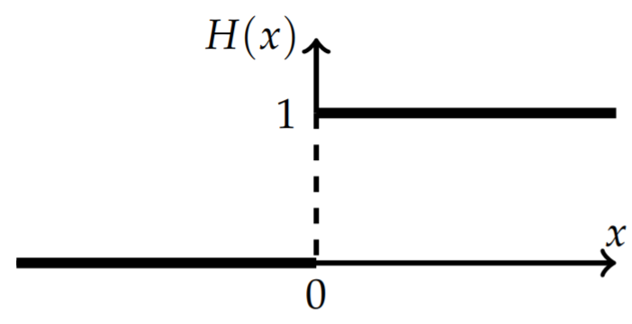
For \(x=\xi\), we have seen that the derivative has a jump in its value. This is similar to the step, or Heaviside, function, \[H(x)= \begin{cases}1, & x>0, \\ 0, & x<0 .\end{cases}\nonumber\] The function is shown in Figure \(\PageIndex{1}\) and we see that the derivative of the step function is zero everywhere except at the jump, or discontinuity. At the jump, there is an infinite slope, though technically, we have learned that there is no derivative at this point. We will try to remedy this situation by introducing the Dirac delta function, \[\delta(x)=\frac{d}{d x} H(x) .\nonumber \] We will show that the Green’s function satisfies the differential equation \[\frac{\partial}{\partial x}\left(p(x) \frac{\partial G(x, \xi)}{\partial x}\right)+q(x) G(x, \xi)=\delta(x-\xi)\label{eq:19}\] However, we will first indicate why this knowledge is useful for the general theory of solving differential equations using Green’s functions.

Figure \(\PageIndex{1}\): The Heaviside step function, \(H(x)\).

Note

The Dirac delta function is described in more detail in Section 9.4. The key property we will need here is the sifting property, \[\int_{a}^{b} f(x) \delta(x-\xi) d x=f(\xi)\nonumber \] for \(a<\xi<b\) .

As noted, the Green’s function satisfies the differential equation \[\frac{\partial}{\partial x}\left(p(x) \frac{\partial G(x, \xi)}{\partial x}\right)+q(x) G(x, \xi)=\delta(x-\xi)\label{eq:20}\] and satisfies homogeneous conditions. We will use the Green’s function to solve the nonhomogeneous equation \[\frac{d}{d x}\left(p(x) \frac{d y(x)}{d x}\right)+q(x) y(x)=f(x) .\label{eq:21}\] These equations can be written in the more compact forms \[\begin{array}{r} \mathcal{L}[y]=f(x) \\ \mathcal{L}[G]=\delta(x-\xi) . \end{array}\label{eq:22}\]

Using these equations, we can determine the solution, \(y(x)\), in terms of the Green’s function. Multiplying the first equation by \(G(x, \xi)\), the second equation by \(y(x)\), and then subtracting, we have \[G \mathcal{L}[y]-y \mathcal{L}[G]=f(x) G(x, \xi)-\delta(x-\xi) y(x) .\nonumber \] Now, integrate both sides from \(x=a\) to \(x=b\). The left hand side becomes \[\int_{a}^{b}[f(x) G(x, \xi)-\delta(x-\xi) y(x)] d x=\int_{a}^{b} f(x) G(x, \xi) d x-y(\xi) .\nonumber \] Using Green’s Identity from Section 4.2.2, the right side is \[\int_{a}^{b}(G \mathcal{L}[y]-y \mathcal{L}[G]) d x=\left[p(x)\left(G(x, \xi) y^{\prime}(x)-y(x) \frac{\partial G}{\partial x}(x, \xi)\right)\right]_{x=a}^{x=b} .\nonumber \] Combining these results and rearranging, we obtain \[\begin{align} y(\xi)=& \int_{a}^{b} f(x) G(x, \xi) d x\nonumber \\ &+\left[p(x)\left(y(x) \frac{\partial G}{\partial x}(x, \xi)-G(x, \xi) y^{\prime}(x)\right)\right]_{x=a}^{x=b} . \label{eq:23} \end{align}\]

Note

Recall that Green’s identity is given by \[\int_{a}^{b}(u \mathcal{L} v-v \mathcal{L} u) d x=\left[p\left(u v^{\prime}-v u^{\prime}\right)\right]_{a}^{b}\nonumber \] The general solution in terms of the boundary value Green’s function with corresponding surface terms.

We will refer to the extra terms in the solution, \[S(b, \tilde{\xi})-S(a, \tilde{\xi})=\left[p(x)\left(y(x) \frac{\partial G}{\partial x}(x, \tilde{\xi})-G(x, \xi) y^{\prime}(x)\right)\right]_{x=a}^{x=b},\nonumber \] as the boundary, or surface, terms. Thus, \[y(\tilde{\zeta})=\int_{a}^{b} f(x) G(x, \xi) d x-[S(b, \tilde{\zeta})-S(a, \xi)] .\nonumber \]

The result in Equation \(\eqref{eq:23}\) is the key equation in determining the solution of a nonhomogeneous boundary value problem. The particular set of boundary conditions in the problem will dictate what conditions \(G(x, \xi)\) has to satisfy. For example, if we have the boundary conditions \(y(a)=0\) and \(y(b)=0\), then the boundary terms yield \[\begin{align} y(\xi)=& \int_{a}^{b} f(x) G(x, \tilde{}) d x-\left[p(b)\left(y(b) \frac{\partial G}{\partial x}(b, \xi)-G(b, \xi) y^{\prime}(b)\right)\right]\nonumber \\ &+\left[p(a)\left(y(a) \frac{\partial G}{\partial x}(a, \xi)-G(a, \xi) y^{\prime}(a)\right)\right]\nonumber \\ =& \int_{a}^{b} f(x) G(x, \xi) d x+p(b) G(b, \xi) y^{\prime}(b)-p(a) G(a, \xi) y^{\prime}(a) .\label{eq:24} \end{align}\] The right hand side will only vanish if \(G(x, \xi)\) also satisfies these homogeneous boundary conditions. This then leaves us with the solution \[y(\xi)=\int_{a}^{b} f(x) G(x, \xi) d x\nonumber \]

We should rewrite this as a function of \(x\). So, we replace \(\xi\) with \(x\) and \(x\) with \(\xi\). This gives \[y(x)=\int_{a}^{b} f(\xi) G(\xi, x) d \xi \text {. }\nonumber \] However, this is not yet in the desirable form. The arguments of the Green’s function are reversed. But, in this case \(G(x, \xi)\) is symmetric in its arguments. So, we can simply switch the arguments getting the desired result.

We can now see that the theory works for other boundary conditions. If we had \(y^{\prime}(a)=0\), then the \(y(a) \frac{\partial G}{d x}(a, \xi)\) term in the boundary terms could be made to vanish if we set \(\frac{\partial G}{\partial x}(a, \xi)=0\). So, this confirms that other boundary value problems can be posed besides the one elaborated upon in the chapter so far.

We can even adapt this theory to nonhomogeneous boundary conditions. We first rewrite Equation \(\eqref{eq:23}\) as \[y(x)=\int_{a}^{b} G(x, \xi) f(\xi) d \xi-\left[p(\xi)\left(y(\xi) \frac{\partial G}{\partial \xi}(x, \xi)-G(x, \xi) y^{\prime}(\xi)\right)\right]_{\tilde = a}^{\tilde{\zeta}=b} .\label{eq:25}\] Let’s consider the boundary conditions \(y(a)=\alpha\) and \(y^{\prime}(b)=\beta\). We also assume that \(G(x, \xi)\) satisfies homogeneous boundary conditions, \[G(a, \xi)=0, \quad \frac{\partial G}{\partial \xi}(b, \xi)=0 .\nonumber \] in both \(x\) and \(\xi\) since the Green’s function is symmetric in its variables. Then, we need only focus on the boundary terms to examine the effect on the solution. We have \[\begin{align} S(b, x)-S(a, x)=&\left[p(b)\left(y(b) \frac{\partial G}{\partial \xi}(x, b)-G(x, b) y^{\prime}(b)\right)\right]\nonumber \\ &-\left[p(a)\left(y(a) \frac{\partial G}{\partial \xi}(x, a)-G(x, a) y^{\prime}(a)\right)\right]\nonumber \\ =&-\beta p(b) G(x, b)-\alpha p(a) \frac{\partial G}{\partial \xi}(x, a) .\label{eq:26} \end{align}\] Therefore, we have the solution \[y(x)=\int_{a}^{b} G(x, \xi) f(\xi) d \xi+\beta p(b) G(x, b)+\alpha p(a) \frac{\partial G}{\partial \xi}(x, a) .\label{eq:27}\] This solution satisfies the nonhomogeneous boundary conditions.

Note

General solution satisfying the nonhomogeneous boundary conditions \(y(a)=\) \(\alpha\) and \(y^{\prime}(b)=\beta\). Here the Green’s function satisfies homogeneous boundary conditions, \(G(a, \xi)=0, \quad \frac{\partial G}{\partial \xi}(b, \xi)=0\).

Example \(\PageIndex{4}\)

Solve \(y^{\prime \prime}=x^{2}, \quad y(0)=1, y(1)=2\) using the boundary value Green’s function.

Solution

This is a modification of Example \(\PageIndex{1}\). We can use the boundary value Green’s function that we found in that problem, \[G(x, \xi)= \begin{cases}-\tilde{\xi}(1-x), & 0 \leq \xi \leq x, \\ -x(1-\xi), & x \leq \xi \leq 1\end{cases}\label{eq:28}\]

We insert the Green’s function into the general solution \(\eqref{eq:27}\) and use the given boundary conditions to obtain \[\begin{align} y(x) &=\int_{0}^{1} G(x, \xi) \tilde{\xi}^{2} d \xi-\left[y(\xi) \frac{\partial G}{\partial \xi}(x, \xi)-G(x, \xi) y^{\prime}(\xi)\right]_{\tilde = 0}^{\tilde{\zeta}=1}\nonumber \\ &=\int_{0}^{x}(x-1) \xi^{3} d \tilde{\xi}+\int_{x}^{1} x(\xi-1) \xi^{2} d \tilde{\xi}+y(0) \frac{\partial G}{\partial \xi}(x, 0)-y(1) \frac{\partial G}{\partial \xi}(x, 1)\nonumber \\ &=\frac{(x-1) x^{4}}{4}+\frac{x\left(1-x^{4}\right)}{4}-\frac{x\left(1-x^{3}\right)}{3}+(x-1)-2 x\nonumber \\ &=\frac{x^{4}}{12}+\frac{35}{12} x-1 .\label{eq:29} \end{align}\]

Of course, this problem can be solved by direct integration. The general solution is \[y(x)=\frac{x^{4}}{12}+c_{1} x+c_{2} .\nonumber \] Inserting this solution into each boundary condition yields the same result.

Note

The Green’s function satisfies a delta function forced differential equation.

We have seen how the introduction of the Dirac delta function in the differential equation satisfied by the Green’s function, Equation \(\eqref{eq:20}\), can lead to the solution of boundary value problems. The Dirac delta function also aids in the interpretation of the Green’s function. We note that the Green’s function is a solution of an equation in which the nonhomogeneous function is \(\delta(x-\xi)\). Note that if we multiply the delta function by \(f(\xi)\) and integrate, we obtain \[\int_{-\infty}^{\infty} \delta(x-\xi) f(\xi) d \xi=f(x)\nonumber\] We can view the delta function as a unit impulse at \(x=\xi\) which can be used to build \(f(x)\) as a sum of impulses of different strengths, \(f(\xi)\). Thus, the Green’s function is the response to the impulse as governed by the differential equation and given boundary conditions.

Note

Derivation of the jump condition for the Green’s function.

In particular, the delta function forced equation can be used to derive the jump condition. We begin with the equation in the form \[\frac{\partial}{\partial x}\left(p(x) \frac{\partial G(x, \xi)}{\partial x}\right)+q(x) G(x, \xi)=\delta(x-\xi) .\label{eq:30}\] Now, integrate both sides from \(\xi-\epsilon\) to \(\xi+\epsilon\) and take the limit as \(\epsilon \rightarrow 0\). Then, \[\begin{align}\lim_{\epsilon\to 0}\int_{\xi-\epsilon}^{\xi+\epsilon}\left[\frac{\partial}{\partial x}\left( p(x)\frac{\partial G(x,\xi)}{\partial x}\right)+q(x)G(x,\xi )\right] dx&=\lim_{\epsilon\to 0}\int_{\xi -\epsilon}^{\xi +\epsilon }\delta (x-\xi )dx\nonumber \\ &=1.\label{eq:31}\end{align}\] Since the \(q(x)\) term is continuous, the limit as \(\epsilon \rightarrow 0\) of that term vanishes. Using the Fundamental Theorem of Calculus, we then have \[\lim _{\epsilon \rightarrow 0}\left[p(x) \frac{\partial G(x, \xi)}{\partial x}\right]_{\tilde{\zeta}-\epsilon}^{\tilde{\xi}+\epsilon}=1 .\label{eq:32}\] This is the jump condition that we have been using!

Series Representations of Green’s Functions

There are times that it might not be so simple to find the Green’s function in the simple closed form that we have seen so far. However, there is a method for determining the Green’s functions of Sturm-Liouville boundary value problems in the form of an eigenfunction expansion. We will finish our discussion of Green’s functions for ordinary differential equations by showing how one obtains such series representations. (Note that we are really just repeating the steps towards developing eigenfunction expansion which we had seen in Section 4.3.)

We will make use of the complete set of eigenfunctions of the differential operator, \(\mathcal{L}\), satisfying the homogeneous boundary conditions: \[\mathcal{L}\left[\phi_{n}\right]=-\lambda_{n} \sigma \phi_{n}, \quad n=1,2, \ldots\nonumber \]

We want to find the particular solution \(y\) satisfying \(\mathcal{L}[y]=f\) and homogeneous boundary conditions. We assume that \[y(x)=\sum_{n=1}^{\infty} a_{n} \phi_{n}(x) .\nonumber \] Inserting this into the differential equation, we obtain \[\mathcal{L}[y]=\sum_{n=1}^{\infty} a_{n} \mathcal{L}\left[\phi_{n}\right]=-\sum_{n=1}^{\infty} \lambda_{n} a_{n} \sigma \phi_{n}=f .\nonumber \]

This has resulted in the generalized Fourier expansion \[f(x)=\sum_{n=1}^{\infty} c_{n} \sigma \phi_{n}(x)\nonumber \] with coefficients \[c_{n}=-\lambda_{n} a_{n} .\nonumber \] We have seen how to compute these coefficients earlier in section 4.3. We multiply both sides by \(\phi_{k}(x)\) and integrate. Using the orthogonality of the eigenfunctions, \[\int_{a}^{b} \phi_{n}(x) \phi_{k}(x) \sigma(x) d x=N_{k} \delta_{n k},\nonumber \] one obtains the expansion coefficients (if \(\lambda_{k} \neq 0\) ) \[a_{k}=-\frac{\left(f, \phi_{k}\right)}{N_{k} \lambda_{k}}\nonumber \] where \(\left(f, \phi_{k}\right) \equiv \int_{a}^{b} f(x) \phi_{k}(x) d x\).

As before, we can rearrange the solution to obtain the Green’s function. Namely, we have \[y(x)=\sum_{n=1}^{\infty} \frac{\left(f, \phi_{n}\right)}{-N_{n} \lambda_{n}} \phi_{n}(x)=\int_{a}^{b} \underbrace{\sum_{n=1}^{\infty} \frac{\phi_{n}(x) \phi_{n}(\xi)}{-N_{n} \lambda_{n}}}_{G(x, \zeta)} f(\xi) d \xi\nonumber \]

Therefore, we have found the Green’s function as an expansion in the eigenfunctions: \[G(x, \xi)=\sum_{n=1}^{\infty} \frac{\phi_{n}(x) \phi_{n}(\xi)}{-\lambda_{n} N_{n}}\label{eq:33}\]

We will conclude this discussion with an example. We will solve this problem three different ways in order to summarize the methods we have used in the text.

Example \(\PageIndex{5}\)

Solve \[y^{\prime \prime}+4 y=x^{2}, \quad x \in(0,1), \quad y(0)=y(1)=0\nonumber \] using the Green’s function eigenfunction expansion.

Solution

The Green’s function for this problem can be constructed fairly quickly for this problem once the eigenvale problem is solved. The eigenvalue problem is \[\phi ''(x)+4\phi (x)=-\lambda\phi (x),\nonumber\] where \(\phi(0)=0\) and \(\phi(1)=0\). The general solution is obtained by rewriting the equation as \[\phi^{\prime \prime}(x)+k^{2} \phi(x)=0,\nonumber \] where \[k^{2}=4+\lambda .\nonumber \]

Solutions satisfying the boundary condition at \(x=0\) are of the form \[\phi(x)=A \sin k x .\nonumber \] Forcing \(\phi(1)=0\) gives \[0=A \sin k \Rightarrow k=n \pi, \quad k=1,2,3 \ldots .\nonumber \] So, the eigenvalues are \[\lambda_{n}=n^{2} \pi^{2}-4, \quad n=1,2, \ldots\nonumber \] and the eigenfunctions are \[\phi_{n}=\sin n \pi x, \quad n=1,2, \ldots\nonumber \]

We also need the normalization constant, \(N_{n}\). We have that \[N_{n}=\left\|\phi_{n}\right\|^{2}=\int_{0}^{1} \sin ^{2} n \pi x=\frac{1}{2} .\nonumber \]

We can now construct the Green’s function for this problem using Equation \(\eqref{eq:33}\). \[G(x, \xi)=2 \sum_{n=1}^{\infty} \frac{\sin n \pi x \sin n \pi \xi}{\left(4-n^{2} \pi^{2}\right)}\label{eq:34}\]

Using this Green’s function, the solution of the boundary value problem becomes \[\begin{align} y(x) &=\int_{0}^{1} G(x, \xi) f(\xi) d \xi\nonumber \\ &=\int_{0}^{1}\left(2 \sum_{n=1}^{\infty} \frac{\sin n \pi x \sin n \pi \tilde{\xi}}{\left(4-n^{2} \pi^{2}\right)}\right) \tilde{\xi}^{2} d \xi\nonumber \\ &=2 \sum_{n=1}^{\infty} \frac{\sin n \pi x}{\left(4-n^{2} \pi^{2}\right)} \int_{0}^{1} \xi^{2} \sin n \pi \xi d \xi\nonumber \\ &=2 \sum_{n=1}^{\infty} \frac{\sin n \pi x}{\left(4-n^{2} \pi^{2}\right)}\left[\frac{\left(2-n^{2} \pi^{2}\right)(-1)^{n}-2}{n^{3} \pi^{3}}\right]\label{eq:35} \end{align}\]

We can compare this solution to the one we would obtain if we did not employ Green’s functions directly. The eigenfunction expansion method for solving boundary value problems, which we saw earlier is demonstrated in the next example.

Example \(\PageIndex{6}\)

Solve \[y^{\prime \prime}+4 y=x^{2}, \quad x \in(0,1), \quad y(0)=y(1)=0\nonumber \] using the eigenfunction expansion method.

Solution

We assume that the solution of this problem is in the form \[y(x)=\sum_{n=1}^{\infty} c_{n} \phi_{n}(x) .\nonumber\]

Inserting this solution into the differential equation \(\mathcal{L}[y]=x^{2}\), gives \[\begin{align} x^{2} &=\mathcal{L}\left[\sum_{n=1}^{\infty} c_{n} \sin n \pi x\right]\nonumber \\ &=\sum_{n=1}^{\infty} c_{n}\left[\frac{d^{2}}{d x^{2}} \sin n \pi x+4 \sin n \pi x\right]\nonumber \\ &=\sum_{n=1}^{\infty} c_{n}\left[4-n^{2} \pi^{2}\right] \sin n \pi x\label{eq:36} \end{align}\]

This is a Fourier sine series expansion of \(f(x)=x^{2}\) on \([0,1]\). Namely, \[f(x)=\sum_{n=1}^{\infty} b_{n} \sin n \pi x .\nonumber \] In order to determine the \(c_{n}\) ’s in Equation \(\eqref{eq:36}\), we will need the Fourier sine series expansion of \(x^{2}\) on \([0,1]\). Thus, we need to compute \[\begin{align} b_{n} &=\frac{2}{1} \int_{0}^{1} x^{2} \sin n \pi x\nonumber \\ &=2\left[\frac{\left(2-n^{2} \pi^{2}\right)(-1)^{n}-2}{n^{3} \pi^{3}}\right], \quad n=1,2, \ldots\label{eq:37} \end{align}\] The resulting Fourier sine series is \[x^{2}=2 \sum_{n=1}^{\infty}\left[\frac{\left(2-n^{2} \pi^{2}\right)(-1)^{n}-2}{n^{3} \pi^{3}}\right] \sin n \pi x .\nonumber \]

Inserting this expansion in Equation \(\eqref{eq:36}\), we find \[2 \sum_{n=1}^{\infty}\left[\frac{\left(2-n^{2} \pi^{2}\right)(-1)^{n}-2}{n^{3} \pi^{3}}\right] \sin n \pi x=\sum_{n=1}^{\infty} c_{n}\left[4-n^{2} \pi^{2}\right] \sin n \pi x .\nonumber \] Due to the linear independence of the eigenfunctions, we can solve for the unknown coefficients to obtain \[c_{n}=2 \frac{\left(2-n^{2} \pi^{2}\right)(-1)^{n}-2}{\left(4-n^{2} \pi^{2}\right) n^{3} \pi^{3}} .\nonumber \] Therefore, the solution using the eigenfunction expansion method is \[\begin{align} y(x) &=\sum_{n=1}^{\infty} c_{n} \phi_{n}(x)\nonumber \\ &=2 \sum_{n=1}^{\infty} \frac{\sin n \pi x}{\left(4-n^{2} \pi^{2}\right)}\left[\frac{\left(2-n^{2} \pi^{2}\right)(-1)^{n}-2}{n^{3} \pi^{3}}\right] .\label{eq:38} \end{align}\]

We note that the solution in this example is the same solution as we had obtained using the Green’s function obtained in series form in the previous example.

One remaining question is the following: Is there a closed form for the Green’s function and the solution to this problem? The answer is yes!

Example \(\PageIndex{7}\)

Find the closed form Green’s function for the problem \[y^{\prime \prime}+4 y=x^{2}, \quad x \in(0,1), \quad y(0)=y(1)=0\nonumber \] and use it to obtain a closed form solution to this boundary value problem.

Solution

We note that the differential operator is a special case of the example done in section 7.2. Namely, we pick \(\omega=2\). The Green’s function was already found in that section. For this special case, we have \[G(x, \xi)= \begin{cases}-\frac{\sin 2(1-\xi) \sin 2 x}{2 \sin 2 \sin 2 \xi}, & 0 \leq x \leq \xi, \\ -\frac{\sin 2(1-x) \sin 2}{2 \sin 2}, & \xi \leq x \leq 1 .\end{cases}\label{eq:39}\]

Using this Green’s function, the solution to the boundary value problem is readily computed \[\begin{align} y(x)&=\int_0^1 G(x,\xi )f(\xi )d\xi\nonumber \\ &=-\int_0^x\frac{\sin 2(1-x)\sin 2\xi}{2\sin 2}\xi^2d\xi +\int_x^1\frac{\sin 2(\xi -1)\sin 2x}{2\sin 2}\xi^2 d\xi\nonumber \\ &=-\frac{1}{4\sin 2}\left[ -x^2\sin 2+(1-\cos ^2x)\sin 2+\sin x\cos x(1+\cos 2)\right].\nonumber \\ &=-\frac{1}{4\sin 2}\left[-x^2\sin 2+2\sin^2 x\sin 1\cos 1+2\sin x\cos x\cos^2 1)\right].\nonumber \\ &=-\frac{1}{8\sin 1\cos 1}\left[-x^2\sin 2+2\sin x\cos 1(\sin x\sin 1+\cos x\cos 1)\right].\nonumber \\ &=\frac{x^2}{4}-\frac{\sin x\cos (1-x)}{4\sin 1}.\label{eq:40}\end{align}\]

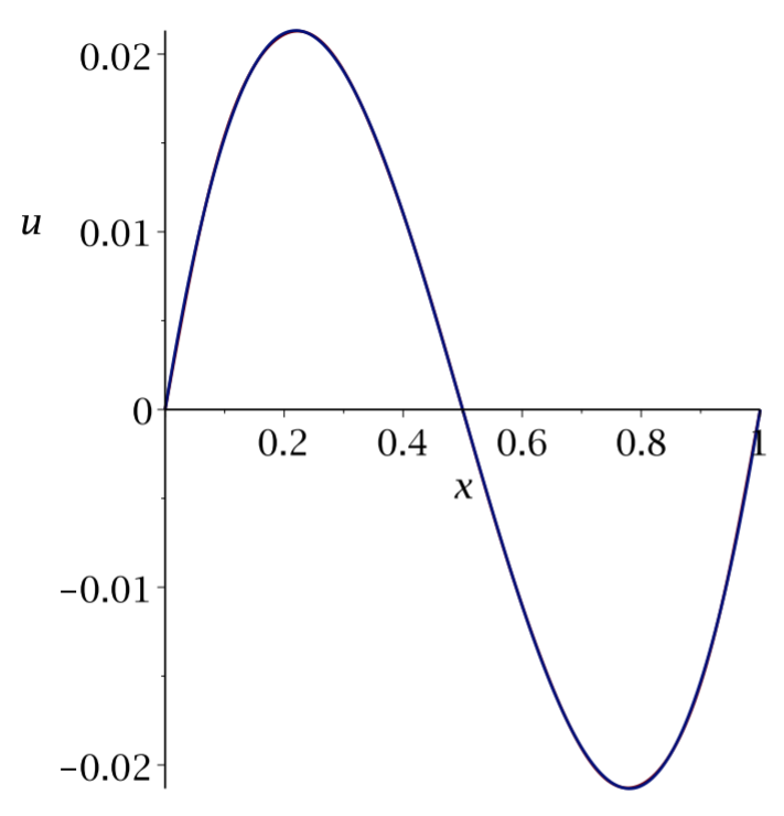
In Figure \(\PageIndex{2}\) we show a plot of this solution along with the first five terms of the series solution. The series solution converges quickly to the closed form solution.

Figure \(\PageIndex{2}\): Plots of the exact solution to Example \(7.6\) with the first five terms of the series solution.

As one last check, we solve the boundary value problem directly, as we had done in the last chapter.

Example \(\PageIndex{8}\)

Solve directly: \[y^{\prime \prime}+4 y=x^{2}, \quad x \in(0,1), \quad y(0)=y(1)=0 .\nonumber \]

Solution

The problem has the general solution \[y(x)=c_{1} \cos 2 x+c_{2} \sin 2 x+y_{p}(x)\nonumber \] where \(y_{p}\) is a particular solution of the nonhomogeneous differential equation. Using the Method of Undetermined Coefficients, we assume a solution of the form \[y_{p}(x)=A x^{2}+B x+C .\nonumber \]

Inserting this guess into the nonhomogeneous equation, we have \[2 A+4\left(A x^{2}+B x+C\right)=x^{2},\nonumber \] Thus, \(B=0,4 A=1\) and \(2 A+4 C=0\). The solution of this system is \[A=\frac{1}{4}, \quad B=0, \quad C=-\frac{1}{8} .\nonumber \] So, the general solution of the nonhomogeneous differential equation is \[y(x)=c_{1} \cos 2 x+c_{2} \sin 2 x+\frac{x^{2}}{4}-\frac{1}{8} .\nonumber \]

We next determine the arbitrary constants using the boundary conditions. We have \[\begin{align} 0 &=y(0)\nonumber \\ &=c_{1}-\frac{1}{8}\nonumber \\ 0 &=y(1)\nonumber \\ &=c_{1} \cos 2+c_{2} \sin 2+\frac{1}{8}\label{eq:41} \end{align}\] Thus, \(c_{1}=\frac{1}{8}\) and \[c_{2}=-\frac{\frac{1}{8}+\frac{1}{8} \cos 2}{\sin 2} .\nonumber \]

Inserting these constants into the solution we find the same solution as before. \[\begin{align} y(x) &=\frac{1}{8} \cos 2 x-\left[\frac{\frac{1}{8}+\frac{1}{8} \cos 2}{\sin 2}\right] \sin 2 x+\frac{x^{2}}{4}-\frac{1}{8}\nonumber \\ &=\frac{(\cos 2 x-1) \sin 2-\sin 2 x(1+\cos 2)}{8 \sin 2}+\frac{x^{2}}{4}\nonumber \\ &=\frac{\left(-2 \sin ^{2} x\right) 2 \sin 1 \cos 1-\sin 2 x\left(2 \cos ^{2} 1\right)}{16 \sin 1 \cos 1}+\frac{x^{2}}{4}\nonumber \\ &=-\frac{\left(\sin ^{2} x\right) \sin 1+\sin x \cos x(\cos 1)}{4 \sin 1}+\frac{x^{2}}{4}\nonumber \\ &=\frac{x^{2}}{4}-\frac{\sin x \cos (1-x)}{4 \sin 1} .\label{eq:42} \end{align}\]

Generalized Green’s Function

When solving \(L u=f\) using eigenfunction expansions, there can be a problem when there are zero eigenvalues. Recall from Section 4.3 the solution of this problem is given by \[\begin{align} y(x) &=\sum_{n=1}^{\infty} c_{n} \phi_{n}(x),\nonumber \\ c_{n} &=-\frac{\int_{a}^{b} f(x) \phi_{n}(x) d x}{\lambda_{m} \int_{a}^{b} \phi_{n}^{2}(x) \sigma(x) d x} .\label{eq:43} \end{align}\] Here the eigenfunctions, \(\phi_{n}(x)\), satisfy the eigenvalue problem \[\mathcal{L} \phi_{n}(x)=-\lambda_{n} \sigma(x) \phi_{n}(x), \quad x \in[a, b]\nonumber \] subject to given homogeneous boundary conditions.

Note that if \(\lambda_{m}=0\) for some value of \(n=m\), then \(c_{m}\) is undefined. However, if we require \[\left(f, \phi_{m}\right)=\int_{a}^{b} f(x) \phi_{n}(x) d x=0,\nonumber \] then there is no problem. This is a form of the Fredholm Alternative. Namely, if \(\lambda_{n}=0\) for some \(n\), then there is no solution unless \(\left.f, \phi_{m}\right)=0\); i.e., \(f\) is orthogonal to \(\phi_{n}\). In this case, \(a_{n}\) will be arbitrary and there are an infinite number of solutions.

Example \(\PageIndex{9}\)

\(u^{\prime \prime}=f(x), u^{\prime}(0)=0, u^{\prime}(L)=0\).

Solution

The eigenfunctions satisfy \(\phi_{n}^{\prime \prime}(x)=-\lambda_{n} \phi_{n}(x), \phi_{n}^{\prime}(0)=0, \phi_{n}^{\prime}(L)=0\). There are the usual solutions, \[\phi_{n}(x)=\cos \frac{n \pi x}{L}, \quad \lambda_{n}=\left(\frac{n \pi}{L}\right)^{2}, \quad n=1,2, \ldots .\nonumber \]

However, when \(\lambda_{n}=0, \phi_{0}^{\prime \prime}(x)=0 .\) So, \(\phi_{0}(x)=A x+B\). The boundary conditions are satisfied if \(A=0\). So, we can take \(\phi_{0}(x)=1\). Therefore, there exists an eigenfunction corresponding to a zero eigenvalue. Thus, in order to have a solution, we have to require \[\int_{0}^{L} f(x) d x=0 .\nonumber \]

Example \(\PageIndex{10}\)

\(u^{\prime \prime}+\pi^{2} u=\beta+2 x, u(0)=0, u(1)=0\).

Solution

In this problem we check to see if there is an eigenfunctions with a zero eigenvalue. The eigenvalue problem is \[\phi^{\prime \prime}+\pi^{2} \phi=0, \quad \phi(0)=0, \quad \phi(1)=0 .\nonumber \] A solution satisfying this problem is easily founds as \[\phi(x)=\sin \pi x .\nonumber \] Therefore, there is a zero eigenvalue. For a solution to exist, we need to require \[\begin{align} 0 &=\int_{0}^{1}(\beta+2 x) \sin \pi x d x\nonumber \\ &=-\left.\frac{\beta}{\pi} \cos \pi x\right|_{0} ^{1}+2\left[\frac{1}{\pi} x \cos \pi x-\frac{1}{\pi^{2}} \sin \pi x\right]_{0}^{1}\nonumber \\ &=-\frac{2}{\pi}(\beta+1) .\label{eq:44} \end{align}\] Thus, either \(\beta=-1\) or there are no solutions.

Recall the series representation of the Green’s function for a Sturm-Liouville problem in Equation \(\eqref{eq:33}\), \[G(x, \zeta)=\sum_{n=1}^{\infty} \frac{\phi_{n}(x) \phi_{n}(\xi)}{-\lambda_{n} N_{n}}\label{eq:45}\] We see that if there is a zero eigenvalue, then we also can run into trouble as one of the terms in the series is undefined.

Recall that the Green’s function satisfies the differential equation \(L G(x, \xi)=\) \(\delta(x-\xi), x, \xi \in[a, b]\) and satisfies some appropriate set of boundary conditions. Using the above analysis, if there is a zero eigenvalue, then \(L \phi_{h}(x)=\) 0 . In order for a solution to exist to the Green’s function differential equation, then \(f(x)=\delta(x-\xi)\) and we have to require \[0=\left(f, \phi_{h}\right)=\int_{a}^{b} \phi_{h}(x) \delta(x-\xi) d x=\phi_{h}(\xi),\nonumber \] for and \(\xi \in[a, b]\). Therefore, the Green’s function does not exist.

We can fix this problem by introducing a modified Green’s function. Let’s consider a modified differential equation, \[L G_{M}(x, \xi)=\delta(x-\xi)+c \phi_{h}(x)\nonumber \] for some constant \(c\). Now, the orthogonality condition becomes \[\begin{align} 0=\left(f, \phi_{h}\right) &=\int_{a}^{b} \phi_{h}(x)\left[\delta(x-\xi)+c \phi_{h}(x)\right] d x\nonumber \\ &=\phi_{h}(\xi)+c \int_{a}^{b} \phi_{h}^{2}(x) d x .\label{eq:46} \end{align}\] Thus, we can choose \[c=-\frac{\phi_{h}(\xi)}{\int_{a}^{b} \phi_{h}^{2}(x) d x}\nonumber \]

Using the modified Green’s function, we can obtain solutions to \(L u=f\). We begin with Green’s identity from Section 4.2.2, given by \[\int_{a}^{b}(u \mathcal{L} v-v \mathcal{L} u) d x=\left[p\left(u v^{\prime}-v u^{\prime}\right)\right]_{a}^{b} .\nonumber \] Letting \(v=G_{M}\), we have \[\int_{a}^{b}\left(G_{M} \mathcal{L}[u]-u \mathcal{L}\left[G_{M}\right]\right) d x=\left[p(x)\left(G_{M}(x, \xi) u^{\prime}(x)-u(x) \frac{\partial G_{M}}{\partial x}(x, \xi)\right)\right]_{x=a}^{x=b} .\nonumber \] Applying homogeneous boundary conditions, the right hand side vanishes. Then we have \[\begin{align} 0 &=\int_{a}^{b}\left(G_{M}(x, \xi) \mathcal{L}[u(x)]-u(x) \mathcal{L}\left[G_{M}(x, \xi)\right]\right) d x\nonumber \\ &=\int_{a}^{b}\left(G_{M}(x, \xi) f(x)-u(x)\left[\delta(x-\xi)+c \phi_{h}(x)\right]\right) d x\nonumber \\ u(\xi) &=\int_{a}^{b} G_{M}(x, \xi) f(x) d x-c \int_{a}^{b} u(x) \phi_{h}(x) d x .\label{eq:47} \end{align}\] Noting that \(u(x, t)=c_{1} \phi_{h}(x)+u_{p}(x)_{\text {, }}\) the last integral gives \[-c \int_{a}^{b} u(x) \phi_{h}(x) d x=\frac{\phi_{h}(\xi)}{\int_{a}^{b} \phi_{h}^{2}(x) d x} \int_{a}^{b} \phi_{h}^{2}(x) d x=c_{1} \phi_{h}(\xi) .\nonumber \] Therefore, the solution can be written as \[u(x)=\int_{a}^{b} f(\xi) G_{M}(x, \xi) d \tilde{\xi}+c_{1} \phi_{h}(x) .\nonumber \] Here we see that there are an infinite number of solutions when solutions exist.

Example \(\PageIndex{11}\)

Use the modified Green’s function to solve \(u^{\prime \prime}+\pi^{2} u=2 x-1\), \(u(0)=0, u(1)=0\).

Solution

We have already seen that a solution exists for this problem, where we have set \(\beta=-1\) in Example \(\PageIndex{10}\).

We construct the modified Green’s function from the solutions of \[\phi_{n}^{\prime \prime}+\pi^{2} \phi_{n}=-\lambda_{n} \phi_{n}, \quad \phi(0)=0, \quad \phi(1)=0 .\nonumber \] The general solutions of this equation are \[\phi_{n}(x)=c_{1} \cos \sqrt{\pi^{2}+\lambda_{n}} x+c_{2} \sin \sqrt{\pi^{2}+\lambda_{n}} x .\nonumber \] Applying the boundary conditions, we have \(c_{1}=0\) and \(\sqrt{\pi^{2}+\lambda_{n}}=n \pi\). Thus, the eigenfunctions and eigenvalues are \[\phi_{n}(x)=\sin n \pi x, \quad \lambda_{n}=\left(n^{2}-1\right) \pi^{2}, \quad n=1,2,3, \ldots .\nonumber \] Note that \(\lambda_{1}=0\).

The modified Green’s function satisfies \[\frac{d^{2}}{d x^{2}} G_{M}(x, \xi)+\pi^{2} G_{M}(x, \xi)=\delta(x-\xi)+c \phi_{h}(x),\nonumber \] where \[\begin{align} c &=-\frac{\phi_{1}(\xi)}{\int_{0}^{1} \phi_{1}^{2}(x) d x}\nonumber \\ &=-\frac{\sin \pi \xi}{\int_{0}^{1} \sin ^{2} \pi \xi, d x}\nonumber \\ &=-2 \sin \pi \xi .\label{eq:48} \end{align}\]

We need to solve for \(\mathrm{G}_{M}(x, \xi)\). The modified Green’s function satisfies \[\frac{d^{2}}{d x^{2}} G_{M}(x, \xi)+\pi^{2} G_{M}(x, \xi)=\delta(x-\xi)-2 \sin \pi \xi \sin \pi x,\nonumber \] and the boundary conditions \(G_{M}(0, \xi)=0\) and \(G_{M}(1, \xi)=0\). We assume an eigenfunction expansion, \[\mathrm{G}_{M}(x, \xi)=\sum_{n=1}^{\infty} c_{n}(\xi) \sin n \pi x .\nonumber \] Then, \[\begin{align} \delta(x-\xi)-2 \sin \pi \xi^{\tilde{s i n} \pi x} &=\frac{d^{2}}{d x^{2}} G_{M}(x, \tilde{})+\pi^{2} G_{M}(x, \tilde{})\nonumber \\ &=-\sum_{n=1}^{\infty} \lambda_{n} c_{n}(\xi) \sin n \pi x\label{eq:49} \end{align}\]

The coefficients are found as \[\begin{align} -\lambda_{n} c_{n} &=2 \int_{0}^{1}[\delta(x-\xi)-2 \sin \pi \xi \sin \pi x] \sin n \pi x d x\nonumber \\ &=2 \sin n \pi \xi-2 \sin \pi \xi \delta_{n 1} .\label{eq:50} \end{align}\] Therefore, \(c_{1}=0\) and \(c_{n}=2 \sin n \pi \tilde{\xi}\), for \(n>1\).

We have found the modified Green’s function as \[G_{M}(x, \xi)=-2 \sum_{n=2}^{\infty} \frac{\sin n \pi x \sin n \pi \tilde{\xi}}{\lambda_{n}} .\nonumber \] We can use this to find the solution. Namely, we have (for \(c_{1}=0\) ) \[\begin{align} u(x) &=\int_{0}^{1}(2 \xi-1) G_{M}(x, \xi) d \xi\nonumber \\ &=-2 \sum_{n=2}^{\infty} \frac{\sin n \pi x}{\lambda_{n}} \int_{0}^{1}(2 \xi-1) \sin n \pi \xi d x\nonumber \\ &=-2 \sum_{n=2}^{\infty} \frac{\sin n \pi x}{\left(n^{2}-1\right) \pi^{2}}\left[-\frac{1}{n \pi}(2 \xi-1) \cos n \pi \xi+\frac{1}{n^{2} \pi^{2}} \sin n \pi \xi\right]_{0}^{1}\nonumber \\ &=2 \sum_{n=2}^{\infty} \frac{1+\cos n \pi}{n\left(n^{2}-1\right) \pi^{3}} \sin n \pi x .\label{eq:51} \end{align}\]

We can also solve this problem exactly. The general solution is given by \[u(x)=c_{1} \sin \pi x+c_{2} \cos \pi x+\frac{2 x-1}{\pi^{2}} .\nonumber \] Imposing the boundary conditions, we obtain \[u(x)=c_{1} \sin \pi x+\frac{1}{\pi^{2}} \cos \pi x+\frac{2 x-1}{\pi^{2}} .\nonumber \] Notice that there are an infinite number of solutions. Choosing \(c_{1}=0\), we have the particular solution \[u(x)=\frac{1}{\pi^{2}} \cos \pi x+\frac{2 x-1}{\pi^{2}} .\nonumber \]

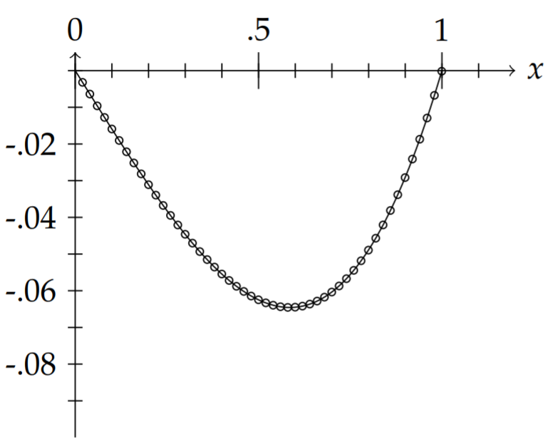
In Figure \(\PageIndex{3}\) we plot this solution and that obtained using the modified Green’s function. The result is that they are in complete agreement.

Figure \(\PageIndex{3}\): The solution for Example \(\PageIndex{11}\).