7.6: Method of Eigenfunction Expansions

We have seen that the use of eigenfunction expansions is another technique for finding solutions of differential equations. In this section we will show how we can use eigenfunction expansions to find the solutions to nonhomogeneous partial differential equations. In particular, we will apply this technique to solving nonhomogeneous versions of the heat and wave equations.

Nonhomogeneous Heat Equation

In this section we solve the one dimensional heat equation with a source using an eigenfunction expansion. Consider the problem \[\begin{align} u_{t} &=k u_{x x}+Q(x, t), \quad 0<x<L, \quad t>0\nonumber \\ u(0, t) &=0, \quad u(L, t)=0, \quad t>0\nonumber \\ u(x, 0) &=f(x), \quad 0<x<L\label{eq:1} \end{align}\]

The homogeneous version of this problem is given by \[\begin{align} v_{t} &=k v_{x x}, \quad 0<x<L, \quad t>0,\nonumber \\ v(0, t) &=0, \quad v(L, t)=0 .\label{eq:2} \end{align}\] We know that a separation of variables leads to the eigenvalue problem \[\phi^{\prime \prime}+\lambda \phi=0, \quad \phi(0)=0, \quad \phi(L)=0 .\nonumber \] The eigenfunctions and eigenvalues are given by \[\phi_{n}(x)=\sin \frac{n \pi x}{L}, \quad \lambda_{n}=\left(\frac{n \pi}{L}\right)^{2}, \quad n=1,2,3, \ldots .\nonumber \]

We can use these eigenfunctions to obtain a solution of the nonhomogeneous problem \(\eqref{eq:1}\). We begin by assuming the solution is given by the eigenfunction expansion \[u(x, t)=\sum_{n=1}^{\infty} a_{n}(t) \phi_{n}(x) .\label{eq:3}\] In general, we assume that \(v(x, t)\) and \(\phi_{n}(x)\) satisfy the same boundary conditions and that \(v(x, t)\) and \(v_{x}(x, t)\) are continuous functions.Note that the difference between this eigenfunction expansion and that in Section 4.3 is that the expansion coefficients are functions of time.

In order to carry out the full process, we will also need to expand the initial profile, \(f(x)\), and the source term, \(Q(x, t)\), in the basis of eigenfunctions. Thus, we assume the forms \[\begin{align} f(x) &=u(x, 0)\nonumber \\ &=\sum_{n=1}^{\infty} a_{n}(0) \phi_{n}(x),\label{eq:4} \\ Q(x, t) &=\sum_{n=1}^{\infty} q_{n}(t) \phi_{n}(x) .\label{eq:5} \end{align}\] Recalling from Chapter 4, the generalized Fourier coefficients are given by \[ a_{n}(0)=\frac{\left\langle f, \phi_{n}\right\rangle}{\left\|\phi_{n}\right\|^{2}}=\frac{1}{\left\|\phi_{n}\right\|^{2}} \int_{0}^{L} f(x) \phi_{n}(x) d x,\label{eq:6}\] \[q_{n}(t)=\frac{\left\langle Q, \phi_{n}\right\rangle}{\left\|\phi_{n}\right\|^{2}}=\frac{1}{\left\|\phi_{n}\right\|^{2}} \int_{0}^{L} Q(x, t) \phi_{n}(x) d x .\label{eq:7}\]

The next step is to insert the expansions \(\eqref{eq:3}\) and \(\eqref{eq:5}\) into the nonhomogeneous heat equation \(\eqref{eq:1}\). We first note that \[\begin{align} u_{t}(x, t) &=\sum_{n=1}^{\infty} \dot{a}_{n}(t) \phi_{n}(x),\nonumber \\ u_{x x}(x, t) &=-\sum_{n=1}^{\infty} a_{n}(t) \lambda_{n} \phi_{n}(x) .\label{eq:8} \end{align}\] Inserting these expansions into the heat equation \(\eqref{eq:1}\), we have \[\begin{align} u_{t} &=k u_{x x}+Q(x, t)\nonumber \\ \sum_{n=1}^{\infty} \dot{a}_{n}(t) \phi_{n}(x) &=-k \sum_{n=1}^{\infty} a_{n}(t) \lambda_{n} \phi_{n}(x)+\sum_{n=1}^{\infty} q_{n}(t) \phi_{n}(x) .\label{eq:9} \end{align}\]

Collecting like terms, we have \[\sum_{n=1}^{\infty}\left[\dot{a}_{n}(t)+k \lambda_{n} a_{n}(t)-q_{n}(t)\right] \phi_{n}(x)=0, \quad \forall x \in[0, L] .\nonumber \] Due to the linear independence of the eigenfunctions, we can conclude that \[\dot{a}_{n}(t)+k \lambda_{n} a_{n}(t)=q_{n}(t), \quad n=1,2,3, \ldots \text {. }\nonumber \] This is a linear first order ordinary differential equation for the unknown expansion coefficients.

We further note that the initial condition can be used to specify the initial condition for this first order ODE. In particular, \[f(x)=\sum_{n=1}^{\infty} a_{n}(0) \phi_{n}(x) .\nonumber \] The coefficients can be found as generalized Fourier coefficients in an expansion of \(f(x)\) in the basis \(\phi_{n}(x)\). These are given by Equation \(\eqref{eq:6}\).

Recall from Appendix B that the solution of a first order ordinary differential equation of the form \[y^{\prime}(t)+a(t) y(t)=p(t)\nonumber \] is found using the integrating factor \[\mu(t)=\exp \int^{t} a(\tau) d \tau .\nonumber \] Multiplying the ODE by the integrating factor, one has \[\frac{d}{d t}\left[y(t) \exp \int^{t} a(\tau) d \tau\right]=p(t) \exp \int^{t} a(\tau) d \tau .\nonumber \] After integrating, the solution can be found providing the integral is doable.

For the current problem, we have \[\dot{a}_{n}(t)+k \lambda_{n} a_{n}(t)=q_{n}(t), \quad n=1,2,3, \ldots .\nonumber \] Then, the integrating factor is \[\mu(t)=\exp \int^{t} k \lambda_{n} d \tau=e^{k \lambda_{n} t} .\nonumber \]

Multiplying the differential equation by the integrating factor, we find \[\begin{align} \left[\dot{a}_{n}(t)+k \lambda_{n} a_{n}(t)\right] e^{k \lambda_{n} t} &=q_{n}(t) e^{k \lambda_{n} t}\nonumber \\ \frac{d}{d t}\left(a_{n}(t) e^{k \lambda_{n} t}\right) &=q_{n}(t) e^{k \lambda_{n} t} .\label{eq:10} \end{align}\]

Integrating, we have \[a_{n}(t) e^{k \lambda_{n} t}-a_{n}(0)=\int_{0}^{t} q_{n}(\tau) e^{k \lambda_{n} \tau} d \tau,\nonumber \] or \[a_{n}(t)=a_{n}(0) e^{-k \lambda_{n} t}+\int_{0}^{t} q_{n}(\tau) e^{-k \lambda_{n}(t-\tau)} d \tau .\nonumber \]

Using these coefficients, we can write out the general solution. \[\begin{align} u(x, t) &=\sum_{n=1}^{\infty} a_{n}(t) \phi_{n}(x)\nonumber \\ &=\sum_{n=1}^{\infty}\left[a_{n}(0) e^{-k \lambda_{n} t}+\int_{0}^{t} q_{n}(\tau) e^{-k \lambda_{n}(t-\tau)} d \tau\right] \phi_{n}(x) .\label{eq:11} \end{align}\]

We will apply this theory to a more specific problem which not only has a heat source but also has nonhomogeneous boundary conditions.

Example \(\PageIndex{1}\)

Solve the following nonhomogeneous heat problem using eigenfunction expansions: \[\begin{align} u_{t}-u_{x x} &=x+t \sin 3 \pi x, \quad 0 \leq x \leq 1, \quad t>0\nonumber \\ u(0, t) &=2, \quad u(L, t)=t, \quad t>0\nonumber \\ u(x, 0) &=3 \sin 2 \pi x+2(1-x), \quad 0 \leq x \leq 1\label{eq:12} \end{align}\]

Solution

This problem has the same nonhomogeneous boundary conditions as those in Example 7.3.2. Recall that we can define \[u(x, t)=v(x, t)+2+(t-2) x\nonumber \] to obtain a new problem for \(v(x, t)\). The new problem is \[\begin{align} v_{t}-v_{x x} &=t \sin 3 \pi x, \quad 0 \leq x \leq 1, \quad t>0,\nonumber \\ v(0, t) &=0, \quad v(L, t)=0, \quad t>0,\nonumber \\ v(x, 0) &=3 \sin 2 \pi x, \quad 0 \leq x \leq 1 .\label{eq:13} \end{align}\]

We can now apply the method of eigenfunction expansions to find \(v(x, t)\). The eigenfunctions satisfy the homogeneous problem \[\phi_{n}^{\prime \prime}+\lambda_{n} \phi_{n}=0, \quad \phi_{n}(0)=0, \quad \phi_{n}(1)=0 .\nonumber \] The solutions are \[\phi_{n}(x)=\sin \frac{n \pi x}{L}, \quad \lambda_{n}=\left(\frac{n \pi}{L}\right)^{2}, \quad n=1,2,3, \ldots\nonumber \]

Now, let \[v(x, t)=\sum_{n=1}^{\infty} a_{n}(t) \sin n \pi x .\nonumber \] Inserting \(v(x, t)\) into the PDE, we have \[\sum_{n=1}^{\infty}\left[\dot{a}_{n}(t)+n^{2} \pi^{2} a_{n}(t)\right] \sin n \pi x=t \sin 3 \pi x .\nonumber \]

Due to the linear independence of the eigenfunctions, we can equate the coefficients of the \(\sin n \pi x\) terms. This gives \[\begin{align} \dot{a}_{n}(t)+n^{2} \pi^{2} a_{n}(t) &=0, \quad n \neq 3,\nonumber \\ \dot{a}_{3}(t)+9 \pi^{2} a_{3}(t) &=t, \quad n=3 .\label{eq:14} \end{align}\] This is a system of first order ordinary differential equations. The first set of equations are separable and are easily solved. For \(n \neq 3\), we seek solutions of \[\frac{d}{d t} a_{n}=-n^{2} \pi^{2} a_{n}(t) .\nonumber \] These are given by \[a_{n}(t)=a_{n}(0) e^{-n^{2} \pi^{2} t}, \quad n \neq 3 .\nonumber \]

In the case \(n=3\), we seek solutions of \[\frac{d}{d t} a_{3}+9 \pi^{2} a_{3}(t)=t .\nonumber \] The integrating factor for this first order equation is given by \[\mu(t)=e^{9 \pi^{2} t} .\nonumber \] Multiplying the differential equation by the integrating factor, we have \[\frac{d}{d t}\left(a_{3}(t) e^{9 \pi^{2} t}\right)=t e^{9 \pi^{2} t} .\nonumber \] Integrating, we obtain the solution \[\begin{align} a_{3}(t) &=a_{3}(0) e^{-9 \pi^{2} t}+e^{-9 \pi^{2} t} \int_{0}^{t} \tau e^{9 \pi^{2} \tau} d \tau,\nonumber \\ &=a_{3}(0) e^{-9 \pi^{2} t}+e^{-9 \pi^{2} t}\left[\frac{1}{9 \pi^{2}} \tau e^{9 \pi^{2} \tau}-\frac{1}{\left(9 \pi^{2}\right)^{2}} e^{9 \pi^{2} \tau}\right]_{0}^{t},\nonumber \\ &=a_{3}(0) e^{-9 \pi^{2} t}+\frac{1}{9 \pi^{2}} t-\frac{1}{\left(9 \pi^{2}\right)^{2}}\left[1-e^{-9 \pi^{2} \tau}\right] .\label{eq:15} \end{align}\]

Up to this point, we have the solution \[\begin{align} u(x, t) &=v(x, t)+w(x, t)\nonumber \\ &=\sum_{n=1}^{\infty} a_{n}(t) \sin n \pi x+2+(t-2) x,\label{eq:16} \end{align}\] where \[\begin{align} &a_{n}(t)=a_{n}(0) e^{-n^{2} \pi^{2} t}, \quad n \neq 3\nonumber \\ &a_{3}(t)=a_{3}(0) e^{-9 \pi^{2} t}+\frac{1}{9 \pi^{2}} t-\frac{1}{\left(9 \pi^{2}\right)^{2}}\left[1-e^{-9 \pi^{2} \tau}\right]\label{eq:17} \end{align}\] We still need to find \(a_{n}(0), n=1,2,3, \ldots\).

The initial values of the expansion coefficients are found using the initial condition \[v(x, 0)=3 \sin 2 \pi x=\sum_{n=1}^{\infty} a_{n}(0) \sin n \pi x .\nonumber \] It is clear that we have \(a_{n}(0)=0\) for \(n \neq 2\) and \(a_{2}(0)=3\). Thus, the series for \(v(x, t)\) has two nonvanishing coefficients, \[\begin{align} &a_{2}(t)=3 e^{-4 \pi^{2} t}\nonumber \\ &a_{3}(t)=\frac{1}{9 \pi^{2}} t-\frac{1}{\left(9 \pi^{2}\right)^{2}}\left[1-e^{-9 \pi^{2} \tau}\right] .\label{eq:18} \end{align}\] Therefore, the final solution is given by \[u(x, t)=2+(t-2) x+3 e^{-4 \pi^{2} t} \sin 2 \pi x+\frac{9 \pi^{2} t-\left(1-e^{-9 \pi^{2} \tau}\right)}{81 \pi^{4}} \sin 3 \pi x .\nonumber \]

Forced Vibrating Membrane

We now consider the forced vibrating membrane. A two-dimensional membrane is stretched over some domain \(D\). We assume Dirichlet conditions on the boundary, \(u=0\) on \(\partial D\). The forced membrane can be modeled as \[\begin{align} u_{t t} &=c^{2} \nabla^{2} u+Q(\mathbf{r}, t), \quad \mathbf{r} \in D, \quad t>0,\nonumber \\ u(\mathbf{r}, t) &=0, \quad \mathbf{r} \in \partial D, \quad t>0,\nonumber \\ u(\mathbf{r}, 0) &=f(\mathbf{r}), \quad u_{t}(\mathbf{r}, 0)=g(\mathbf{r}), \quad \mathbf{r} \in D .\label{eq:19} \end{align}\]

The method of eigenfunction expansions relies on the use of eigenfunctions, \(\phi_{\alpha}(\mathbf{r})\), for \(\alpha \in J \subset Z^{2}\) a set of indices typically of the form \((i, j)\) in some lattice grid of integers. The eigenfunctions satisfy the eigenvalue equation \[\nabla^{2} \phi_{\alpha}(\mathbf{r})=-\lambda_{\alpha} \phi_{\alpha}(\mathbf{r}), \quad \phi_{\alpha}(\mathbf{r})=0 \text {, on } \partial D \text {. }\nonumber \]

We assume that the solution and forcing function can be expanded in the basis of eigenfunctions, \[\begin{align} u(\mathbf{r}, t) &=\sum_{\alpha \in J} a_{\alpha}(t) \phi_{\alpha}(\mathbf{r}),\nonumber \\ Q(\mathbf{r}, t) &=\sum_{\alpha \in J} q_{\alpha}(t) \phi_{\alpha}(\mathbf{r}) .\label{eq:20} \end{align}\]

Inserting this form into the forced wave equation \(\eqref{eq:19}\), we have \[\begin{align} u_{t t} &=c^{2} \nabla^{2} u+Q(\mathbf{r}, t)\nonumber \\ \sum_{\alpha \in J} \ddot{a}_{\alpha}(t) \phi_{\alpha}(\mathbf{r}) &=-c^{2} \sum_{\alpha \in J} \lambda_{\alpha} a_{\alpha}(t) \phi_{\alpha}(\mathbf{r})+\sum_{\alpha \in J} q_{\alpha}(t) \phi_{\alpha}(\mathbf{r})\nonumber \\ 0 &=\sum_{\alpha \in J}\left[\ddot{a}_{\alpha}(t)+c^{2} \lambda_{\alpha} a_{\alpha}(t)-q_{\alpha}(t)\right] \phi_{\alpha}(\mathbf{r}) .\label{eq:21} \end{align}\]

The linear independence of the eigenfunctions then gives the ordinary differential equation \[\ddot{a}_{\alpha}(t)+c^{2} \lambda_{\alpha} a_{\alpha}(t)=q_{\alpha}(t) .\nonumber \] We can solve this equation with initial conditions \(a_{\alpha}(0)\) and \(\dot{a}_{\alpha}(0)\) found from \[\begin{align} &f(\mathbf{r})=u(\mathbf{r}, 0)=\sum_{\alpha \in J} a_{\alpha}(0) \phi_{\alpha}(\mathbf{r}),\nonumber \\ &g(\mathbf{r})=u_{t}(\mathbf{r}, 0)=\sum_{\alpha \in J} \dot{a}_{\alpha}(0) \phi_{\alpha}(\mathbf{r}) .\label{eq:22} \end{align}\]

Example \(\PageIndex{2}\)

Periodic Forcing, \(Q(\mathbf{r}, t)=G(\mathbf{r}) \cos \omega t\).

Solution

It is enough to specify \(Q(\mathbf{r}, t)\) in order to solve for the time dependence of the expansion coefficients. A simple example is the case of periodic forcing, \(Q(\mathbf{r}, t)=\) \(h(\mathbf{r}) \cos \omega t\). In this case, we expand \(Q\) in the basis of eigenfunctions, \[\begin{align} Q(\mathbf{r}, t) &=\sum_{\alpha \in J} q_{\alpha}(t) \phi_{\alpha}(\mathbf{r}),\nonumber \\ G(\mathbf{r}) \cos \omega t &=\sum_{\alpha \in J} \gamma_{\alpha} \cos \omega t \phi_{\alpha}(\mathbf{r}) .\label{eq:23} \end{align}\]

Inserting these expressions into the forced wave equation \(\eqref{eq:19}\), we obtain a system of differential equations for the expansion coefficients, \[\ddot{a}_{\alpha}(t)+c^{2} \lambda_{\alpha} a_{\alpha}(t)=\gamma_{\alpha} \cos \omega t .\nonumber \]

In order to solve this equation we borrow the methods from a course on ordinary differential equations for solving nonhomogeneous equations. In particular we can use the Method of Undetermined Coefficients as reviewed in Section B.3.1. The solution of these equations are of the form \[a_{\alpha}(t)=a_{\alpha h}(t)+a_{\alpha p}(t),\nonumber \] where \(a_{\alpha h}(t)\) satisfies the homogeneous equation, \[\ddot{a}_{\alpha h}(t)+c^{2} \lambda_{\alpha} a_{\alpha h}(t)=0,\label{eq:24} \] and \(a_{\alpha p}(t)\) is a particular solution of the nonhomogeneous equation, \[\ddot{a}_{\alpha p}(t)+c^{2} \lambda_{\alpha} a_{\alpha p}(t)=\gamma_{\alpha} \cos \omega t .\label{eq:25}\]

The solution of the homogeneous problem \(\eqref{eq:24}\) is easily founds as \[a_{\alpha h}(t)=c_{1 \alpha} \cos \left(\omega_{0 \alpha} t\right)+c_{2 \alpha} \sin \left(\omega_{0 \alpha} t\right),\nonumber \] where \(\omega_{0 \alpha}=c \sqrt{\lambda_{\alpha}}\).

The particular solution is found by making the guess \(a_{\alpha p}(t)=A_{\alpha} \cos \omega t\). Inserting this guess into Equation (ceqn2), we have \[\left[-\omega^{2}+c^{2} \lambda_{\alpha}\right] A_{\alpha} \cos \omega t=\gamma_{\alpha} \cos \omega t\nonumber \] Solving for \(A_{\alpha}\), we obtain \[A_{\alpha}=\frac{\gamma_{\alpha}}{-\omega^{2}+c^{2} \lambda_{\alpha}}, \quad \omega^{2} \neq c^{2} \lambda_{\alpha} .\nonumber \] Then, the general solution is given by \[a_{\alpha}(t)=c_{1 \alpha} \cos \left(\omega_{0 \alpha} t\right)+c_{2 \alpha} \sin \left(\omega_{0 \alpha} t\right)+\frac{\gamma_{\alpha}}{-\omega^{2}+c^{2} \lambda_{\alpha}} \cos \omega t,\nonumber \] where \(\omega_{0 \alpha}=c \sqrt{\lambda_{\alpha}}\) and \(\omega^{2} \neq c^{2} \lambda_{\alpha}\)

In the case where \(\omega^{2}=c^{2} \lambda_{\alpha}\), we have a resonant solution. This is discussed in Section FO on forced oscillations. In this case the Method of Undetermined Coefficients fails and we need the Modified Method of Undetermined Coefficients. This is because the driving term, \(\gamma_{\alpha} \cos \omega t\), is a solution of the homogeneous problem. So, we make a different guess for the particular solution. We let \[a_{\alpha p}(t)=t\left(A_{\alpha} \cos \omega t+B_{\alpha} \sin \omega t\right) .\nonumber \] Then, the needed derivatives are \[\begin{align} a_{\alpha p}(t) &=\omega t\left(-A_{\alpha} \sin \omega t+B_{\alpha} \cos \omega t\right)+A_{\alpha} \cos \omega t+B_{\alpha} \sin \omega t\nonumber \\ a_{\alpha p}(t) &=-\omega^{2} t\left(A_{\alpha} \cos \omega t+B_{\alpha} \sin \omega t\right)-2 \omega A_{\alpha} \sin \omega t+2 \omega B_{\alpha} \cos \omega t\nonumber \\ &=-\omega^{2} a_{\alpha p}(t)-2 \omega A_{\alpha} \sin \omega t+2 \omega B_{\alpha} \cos \omega t\label{eq:26} \end{align}\]

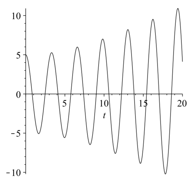
Inserting this guess into Equation (ceqn 2 ) and noting that \(\omega^{2}=c^{2} \lambda_{\alpha}\), we have \[-2 \omega A_{\alpha} \sin \omega t+2 \omega B_{\alpha} \cos \omega t=\gamma_{\alpha} \cos \omega t .\nonumber \] Therefore, \(A_{\alpha}=0\) and \[B_{\alpha}=\frac{\gamma_{\alpha}}{2 \omega} .\nonumber \] So, the particular solution becomes \[a_{\alpha p}(t)=\frac{\gamma_{\alpha}}{2 \omega} t \sin \omega t .\nonumber \] The full general solution is then \[a_{\alpha}(t)=c_{1 \alpha} \cos (\omega t)+c_{2 \alpha} \sin (\omega t)+\frac{\gamma_{\alpha}}{2 \omega} t \sin \omega t,\nonumber \] where \(\omega=c \sqrt{\lambda_{\alpha}}\).

We see from this result that the solution tends to grow as \(t\) gets large. This is what is called a resonance. Essentially, one is driving the system at its natural frequency for one of the frequencies in the system. A typical plot of such a solution in Figure \(\PageIndex{1}\).

Figure \(\PageIndex{1}\): Plot of a solution showing resonance.