9.1: Introduction

Some of the most powerful tools for solving problems in physics are transform methods. The idea is that one can transform the problem at hand to a new problem in a different space, hoping that the problem in the new space is easier to solve. Such transforms appear in many forms.

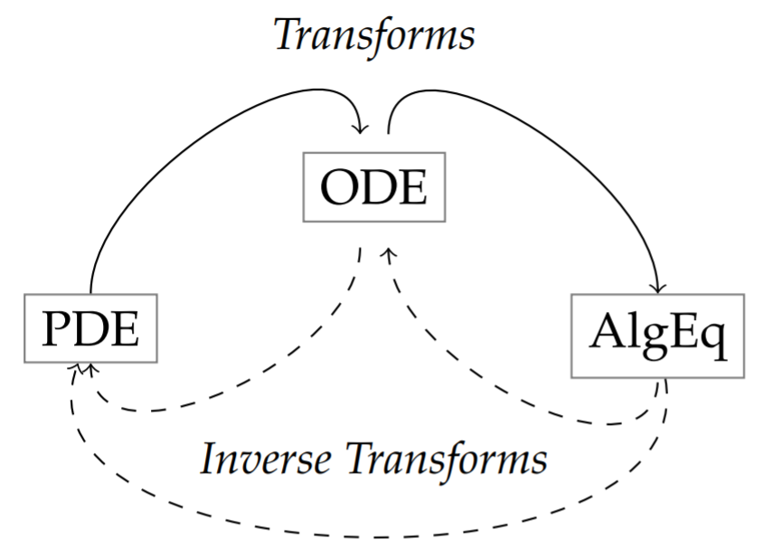
As we had seen in Chapter 3 and will see later in the book, the solutions of linear partial differential equations can be found by using the method of separation of variables to reduce solving partial differential equations (PDEs) to solving ordinary differential equations (ODEs). We can also use transform methods to transform the given PDE into ODEs or algebraic equations. Solving these equations, we then construct solutions of the PDE (or, the ODE) using an inverse transform. A schematic of these processes is shown below and we will describe in this chapter how one can use Fourier and Laplace transforms to this effect.

Figure \(\PageIndex{1}\): Schematic indicating that PDEs and ODEs can be transformed to simpler problems, solved in the new space and transformed back to the original space.

Note

In this chapter we will explore the use of integral transforms. Given a function \(f(x)\), we define an integral transform to a new function \(F(k)\) as \[F(k)=\int_{a}^{b} f(x) K(x, k) d x .\nonumber \] Here \(K(x, k)\) is called the kernel of the transform. We will concentrate specifically on Fourier transforms, \[\hat{f}(k)=\int_{-\infty}^{\infty} f(x) e^{i k x} d x\nonumber \] and Laplace transforms \[F(s)=\int_{0}^{\infty} f(t) e^{-s t} d t .\nonumber \]

Example 1 - The Linearized \(\mathrm{KdV}\) Equation

As a relatively simple example, we consider the linearized Kortewegde Vries (KdV) equation: \[u_{t}+c u_{x}+\beta u_{x x x}=0, \quad-\infty<x<\infty .\label{eq:1}\] This equation governs the propagation of some small amplitude water waves. Its nonlinear counterpart has been at the center of attention in the last 40 years as a generic nonlinear wave equation.

Note

The nonlinear counterpart to this equation is the Korteweg-de Vries (KdV) equation: \(u_{t}+6 u u_{x}+u_{x x x}=0\). This equation was derived by Diederik Johannes Korteweg (1848-1941) and his student Gustav de Vries (1866-1934). This equation governs the propagation of traveling waves called solutons. These were first observed by John Scott Russell (1808-1882) and were the source of a long debate on the existence of such waves. The history of this debate is interesting and the KdV turned up as a generic equation in many other fields in the latter part of the last century leading to many papers on nonlinear evolution equations.

We seek solutions that oscillate in space. So, we assume a solution of the form \[u(x, t)=A(t) e^{i k x} .\label{eq:2}\] Such behavior was seen in Chapters 3 and 6 for the wave equation for vibrating strings. In that case, we found plane wave solutions of the form \(e^{i k(x \pm c t)}\), which we could write as \(e^{i(k x \pm \omega t)}\) by defining \(\omega=k c\). We further note that one often seeks complex solutions as a linear combination of such forms and then takes the real part in order to obtain physical solutions. In this case, we will find plane wave solutions for which the angular frequency \(\omega=\omega(k)\) is a function of the wavenumber.

Inserting the guess \(\eqref{eq:2}\) into the linearized KdV equation, we find that \[\frac{d A}{d t}+i\left(c k-\beta k^{3}\right) A=0 \text {. }\label{eq:3}\] Thus, we have converted the problem of seeking a solution of the partial differential equation into seeking a solution to an ordinary differential equation. This new problem is easier to solve. In fact, given an initial value, \(A(0)\), we have \[A(t)=A(0) e^{-i\left(c k-\beta k^{3}\right) t} .\label{eq:4}\]

Therefore, the solution of the partial differential equation is \[u(x, t)=A(0) e^{i k\left(x-\left(c-\beta k^{2}\right) t\right)} .\label{eq:5}\] We note that this solution takes the form \(e^{i(k x-\omega t)}\), where \[\omega=c k-\beta k^{3} .\nonumber \]

Note

A dispersion relation is an expression giving the angular frequency as a function of the wave number, \(\omega=\omega(k)\).

In general, the equation \(\omega=\omega(k)\) gives the angular frequency as a function of the wave number, \(k\), and is called a dispersion relation. For \(\beta=0\), we see that \(c\) is nothing but the wave speed. For \(\beta \neq 0\), the wave speed is given as \[v=\frac{\omega}{k}=c-\beta k^{2} .\nonumber \] This suggests that waves with different wave numbers will travel at different speeds. Recalling that wave numbers are related to wavelengths, \(k=\frac{2 \pi}{\lambda}\), this means that waves with different wavelengths will travel at different speeds. For example, an initial localized wave packet will not maintain its shape. It is said to disperse, as the component waves of differing wavelengths will tend to part company.

For a general initial condition, we write the solutions to the linearized \(\mathrm{KdV}\) as a superposition of plane waves. We can do this since the partial differential equation is linear. This should remind you of what we had done when using separation of variables. We first sought product solutions and then took a linear combination of the product solutions to obtain the general solution.

For this problem, we will sum over all wave numbers. The wave numbers are not restricted to discrete values. We instead have a continuous range of values. Thus, "summing" over \(k\) means that we have to integrate over the wave numbers. Thus, we have the general solution\(^{1}\) \[u(x, t)=\frac{1}{2 \pi} \int_{-\infty}^{\infty} A(k, 0) e^{i k\left(x-\left(c-\beta k^{2}\right) t\right)} d k .\label{eq:6}\] Note that we have indicated that \(A\) is a function of \(k\). This is similar to introducing the \(A_{n}\) ’s and \(B_{n}\) ’s in the series solution for waves on a string.

Note

The extra \(2 \pi\) has been introduced to be consistent with the definition of the Fourier transform which is given later in the chapter.

How do we determine the \(A(k, 0)\) ’s? We introduce as an initial condition the initial wave profile \(u(x, 0)=f(x)\). Then, we have \[f(x)=u(x, 0)=\frac{1}{2 \pi} \int_{-\infty}^{\infty} A(k, 0) e^{i k x} d k .\label{eq:7}\] Thus, given \(f(x)\), we seek \(A(k, 0)\). In this chapter we will see that \[A(k, 0)=\int_{-\infty}^{\infty} f(x) e^{-i k x} d x\nonumber \] This is what is called the Fourier transform of \(f(x)\). It is just one of the so-called integral transforms that we will consider in this chapter.

In Figure \(\PageIndex{2}\) we summarize the transform scheme. One can use methods like separation of variables to solve the partial differential equation directly, evolving the initial condition \(u(x, 0)\) into the solution \(u(x, t)\) at a later time.

Figure \(\PageIndex{2}\): Schematic of using Fourier transforms to solve a linear evolution equation.

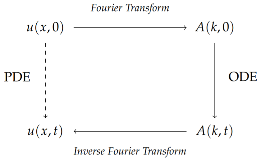
The transform method works as follows. Starting with the initial condition, one computes its Fourier Transform (FT) as\(^{2}\) \[A(k, 0)=\int_{-\infty}^{\infty} f(x) e^{-i k x} d x\nonumber \] Applying the transform on the partial differential equation, one obtains an ordinary differential equation satisfied by \(A(k, t)\) which is simpler to solve than the original partial differential equation. Once \(A(k, t)\) has been found, then one applies the Inverse Fourier Transform (IFT) to \(A(k, t)\) in order to get the desired solution: \[\begin{align} u(x, t) &=\frac{1}{2 \pi} \int_{-\infty}^{\infty} A(k, t) e^{i k x} d k\nonumber \\ &=\frac{1}{2 \pi} \int_{-\infty}^{\infty} A(k, 0) e^{i k\left(x-\left(c-\beta k^{2}\right) t\right)} d k .\label{eq:8} \end{align}\]

Note

The Fourier transform as used in this section and the next section are defined slightly differently than how we will define them later. The sign of the exponentials has been reversed. The one dimensional time dependent Schrödinger equation.

Example 2 - The Free Particle Wave Function

A more familiar example in physics comes from quantum mechanics. The Schrödinger equation gives the wave function \(\Psi(x, t)\) for a particle under the influence of forces, represented through the corresponding potential function \(V(x)\). The one dimensional time dependent Schrödinger equation is given by \[i \hbar \Psi_{t}=-\frac{\hbar^{2}}{2 m} \Psi_{x x}+V \Psi \text {. }\label{eq:9}\] We consider the case of a free particle in which there are no forces, \(V=0\). Then we have \[i \hbar \Psi_{t}=-\frac{\hbar^{2}}{2 m} \Psi_{x x} .\label{eq:10}\]

Taking a hint from the study of the linearized KdV equation, we will assume that solutions of Equation \(\eqref{eq:10}\) take the form \[\Psi(x, t)=\frac{1}{2 \pi} \int_{-\infty}^{\infty} \phi(k, t) e^{i k x} d k .\nonumber \] [Here we have opted to use the more traditional notation, \(\phi(k, t)\) instead of \(A(k, t)\) as above.]

Inserting the expression for \(\Psi(x, t)\) into \(\eqref{eq:10}\), we have \[i \hbar \int_{-\infty}^{\infty} \frac{d \phi(k, t)}{d t} e^{i k x} d k=-\frac{\hbar^{2}}{2 m} \int_{-\infty}^{\infty} \phi(k, t)(i k)^{2} e^{i k x} d k .\nonumber \] Since this is true for all \(t\), we can equate the integrands, giving \[i \hbar \frac{d \phi(k, t)}{d t}=\frac{\hbar^{2} k^{2}}{2 m} \phi(k, t) .\nonumber \] As with the last example, we have obtained a simple ordinary differential equation. The solution of this equation is given by \[\phi(k, t)=\phi(k, 0) e^{-i \frac{\hbar k^{2}}{2 m} t} .\nonumber \] Applying the inverse Fourier transform, the general solution to the time dependent problem for a free particle is found as \[\Psi(x, t)=\frac{1}{2 \pi} \int_{-\infty}^{\infty} \phi(k, 0) e^{i k\left(x-\frac{\hbar k}{2 m} t\right)} d k .\nonumber \] We note that this takes the familiar form \[\Psi(x, t)=\frac{1}{2 \pi} \int_{-\infty}^{\infty} \phi(k, 0) e^{i(k x-\omega t)} d k,\nonumber \] where the dispersion relation is found as \[\omega=\frac{\hbar k^{2}}{2 m} .\nonumber \]

The wave speed is given as \[v=\frac{\omega}{k}=\frac{\hbar k}{2 m} .\nonumber \] As a special note, we see that this is not the particle velocity! Recall that the momentum is given as \(p=\hbar k .\)\(^{3}\) So, this wave speed is \(v=\frac{p}{2 m}\), which is only half the classical particle velocity! A simple manipulation of this result will clarify the "problem."

Note

Since \(p=\hbar k\), we also see that the dispersion relation is given by \[\omega=\frac{\hbar k^{2}}{2 m}=\frac{p^{2}}{2 m \hbar}=\frac{E}{\hbar}\nonumber\]

We assume that particles can be represented by a localized wave function. This is the case if the major contributions to the integral are centered about a central wave number, \(k_{0}\). Thus, we can expand \(\omega(k)\) about \(k_{0}\) : \[\omega(k)=\omega_{0}+\omega_{0}^{\prime}\left(k-k_{0}\right) t+\ldots .\label{eq:11}\] Here \(\omega_{0}=\omega\left(k_{0}\right)\) and \(\omega_{0}^{\prime}=\omega^{\prime}\left(k_{0}\right)\). Inserting this expression into the integral representation for \(\Psi(x, t)\), we have \[\Psi(x, t)=\frac{1}{2 \pi} \int_{-\infty}^{\infty} \phi(k, 0) e^{i\left(k x-\omega_{0} t-\omega_{0}^{\prime}\left(k-k_{0}\right) t-\ldots\right)} d k,\nonumber \] We now make the change of variables, \(s=k-k_{0}\), and rearrange the resulting factors to find \[\begin{align} \Psi(x, t) & \approx \frac{1}{2 \pi} \int_{-\infty}^{\infty} \phi\left(k_{0}+s, 0\right) e^{i\left(\left(k_{0}+s\right) x-\left(\omega_{0}+\omega_{0}^{\prime} s\right) t\right)} d s\nonumber \\ &=\frac{1}{2 \pi} e^{i\left(-\omega_{0} t+k_{0} \omega_{0}^{\prime} t\right)} \int_{-\infty}^{\infty} \phi\left(k_{0}+s, 0\right) e^{i\left(k_{0}+s\right)\left(x-\omega_{0}^{\prime} t\right)} d s\nonumber \\ &=e^{i\left(-\omega_{0} t+k_{0} \omega_{0}^{\prime} t\right)} \Psi\left(x-\omega_{0}^{\prime} t, 0\right) .\label{eq:12} \end{align}\]

Note

Group and phase velocities, \(v_{g}=\frac{d \omega}{d k}\), \(v_{p}=\frac{\omega}{k} .\)

Summarizing, for an initially localized wave packet, \(\Psi(x, 0)\) with wave numbers grouped around \(k_{0}\) the wave function, \(\Psi(x, t)\), is a translated version of the initial wave function up to a phase factor. In quantum mechanics we are more interested in the probability density for locating a particle, so from \[|\Psi(x, t)|^{2}=\left|\Psi\left(x-\omega_{0}^{\prime} t, 0\right)\right|^{2}\nonumber \] we see that the "velocity of the wave packet" is found to be \[\omega_{0}^{\prime}=\left.\frac{d \omega}{d k}\right|_{k=k_{0}}=\frac{\hbar k}{m} .\nonumber \] This corresponds to the classical velocity of the particle \(\left(v_{\text {part }}=p / m\right)\). Thus, one usually defines \(\omega_{0}^{\prime}\) to be the group velocity, \[v_{g}=\frac{d \omega}{d k}\nonumber \] and the former velocity as the phase velocity, \[v_{p}=\frac{\omega}{k} .\nonumber \]

Transform Schemes

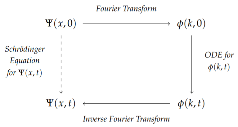
These examples have illustrated one of the features of transform theory. Given a partial differential equation, we can transform the equation from spatial variables to wave number space, or time variables to frequency space. In the new space the time evolution is simpler. In these cases, the evolution was governed by an ordinary differential equation. One solves the problem in the new space and then transforms back to the original space. This is depicted in Figure \(\PageIndex{3}\) for the Schrödinger equation and was shown in Figure \(\PageIndex{2}\) for the linearized \(\mathrm{KdV}\) equation.

Figure \(\PageIndex{3}\): The scheme for solving the Schrödinger equation using Fourier transforms. The goal is to solve for \(\Psi(x, t)\) given \(\Psi(x, 0)\). Instead of a direct solution in coordinate space (on the left side), one can first transform the initial condition obtaining \(\phi(k, 0)\) in wave number space. The governing equation in the new space is found by transforming the PDE to get an ODE. This simpler equation is solved to obtain \(\phi(k, t)\). Then an inverse transform yields the solution of the original equation.

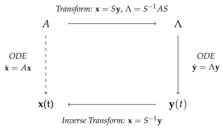
This is similar to the solution of the system of ordinary differential equations in Chapter 3, \(\dot{\mathbf{x}}=A\mathbf{x}\) In that case we diagonalized the system using the transformation \(\mathbf{x} = S\mathbf{y}\). This lead to a simpler system \(\dot{\mathbf{y}} = Λ\mathbf{y}\), where \(Λ = S^{−1}AS\). Solving for \(\mathbf{y}\), we inverted the solution to obtain \(\mathbf{x}\). Similarly, one can apply this diagonalization to the solution of linear algebraic systems of equations. The general scheme is shown in Figure \(\PageIndex{4}\).

Figure \(\PageIndex{4}\): This shows the scheme for solving the linear system of ODEs \(\dot{\mathbf{x}}=\) \(A \mathrm{x}\). One finds a transformation between \(\mathbf{x}\) and \(\mathbf{y}\) of the form \(\mathbf{x}=S \mathbf{y}\) which diagonalizes the system. The resulting system is easier to solve for \(\mathbf{y}\). Then, one uses the inverse transformation to obtain the solution to the original problem.

Similar transform constructions occur for many other type of problems. We will end this chapter with a study of Laplace transforms, which are useful in the study of initial value problems, particularly for linear ordinary differential equations with constant coefficients. A similar scheme for using Laplace transforms is depicted in Figure 9.8.1.

In this chapter we will begin with the study of Fourier transforms. These will provide an integral representation of functions defined on the real line. Such functions can also represent analog signals. Analog signals are continuous signals which can be represented as a sum over a continuous set of frequencies, as opposed to the sum over discrete frequencies, which Fourier series were used to represent in an earlier chapter. We will then investigate a related transform, the Laplace transform, which is useful in solving initial value problems such as those encountered in ordinary differential equations.