9.4: The Dirac Delta Function

In the last section we introduced the Dirac delta function, \(\delta(x)\). As noted above, this is one example of what is known as a generalized function, or a distribution. Dirac had introduced this function in the \(1930^{\prime}\)s in his study of quantum mechanics as a useful tool. It was later studied in a general theory of distributions and found to be more than a simple tool used by physicists. The Dirac delta function, as any distribution, only makes sense under an integral.

Note

P. A. M. Dirac (1902-1984) introduced the \(\delta\) function in his book, The Principles of Quantum Mechanics, 4th Ed., Oxford University Press, 1958, originally published in 1930, as part of his orthogonality statement for a basis of functions in a Hilbert space, \(< \xi '|\xi ''> =c\delta (\xi '-\xi '')\) in the same way we introduced discrete orthogonality using the Kronecker delta.

Two properties were used in the last section. First one has that the area under the delta function is one, \[\int_{-\infty}^{\infty} \delta(x) d x=1 .\nonumber \] Integration over more general intervals gives \[\int_{a}^{b} \delta(x) d x= \begin{cases}1, & 0 \notin[a, b], \\ 0, & 0 \notin[a, b] .\end{cases}\label{eq:1}\]

The other property that was used was the sifting property: \[\int_{-\infty}^{\infty} \delta(x-a) f(x) d x=f(a) \text {. }\nonumber \] This can be seen by noting that the delta function is zero everywhere except at \(x=a\). Therefore, the integrand is zero everywhere and the only contribution from \(f(x)\) will be from \(x=a\). So, we can replace \(f(x)\) with \(f(a)\) under the integral. Since \(f(a)\) is a constant, we have that \[\begin{align} \int_{-\infty}^{\infty} \delta(x-a) f(x) d x &=\int_{-\infty}^{\infty} \delta(x-a) f(a) d x\nonumber \\ &=f(a) \int_{-\infty}^{\infty} \delta(x-a) d x=f(a) .\label{eq:2} \end{align}\]

Note

Properties of the Dirac \(\delta\)-function: \[\begin{gathered} \int_{-\infty}^{\infty} \delta(x-a) f(x) d x=f(a) \\ \int_{-\infty}^{\infty} \delta(a x) d x=\frac{1}{|a|} \int_{-\infty}^{\infty} \delta(y) d y . \\ \int_{-\infty}^{\infty} \delta(f(x)) d x=\int_{-\infty}^{\infty} \sum_{j=1}^{n} \frac{\delta\left(x-x_{j}\right)}{\left|f^{\prime}\left(x_{j}\right)\right|} d x . \end{gathered}\nonumber \] (For \(n\) simple roots.)

These and other properties are often written outside the integral: \[\begin{gathered} \delta(a x)=\frac{1}{|a|} \delta(x) \\ \delta(-x)=\delta(x) \\ \delta((x-a)(x-b))=\frac{[\delta(x-a)+\delta(x-a)]}{|a-b|} \\ (x-b))=\frac{[\delta(x-a)+\delta}{\mid a-b} \\ \delta(f(x))=\sum_{j} \frac{\delta\left(x-x_{j}\right)}{\left|f^{\prime}\left(x_{j}\right)\right|} \end{gathered}\nonumber \] for \(f\left(x_{j}\right)=0, f^{\prime}\left(x_{j}\right) \neq 0 .\)

Another property results from using a scaled argument, \(a x\). In this case we show that \[\delta(a x)=|a|^{-1} \delta(x) .\label{eq:3}\] As usual, this only has meaning under an integral sign. So, we place \(\delta(a x)\) inside an integral and make a substitution \(y=a x\) : \[\begin{align}\int_{-\infty}^{\infty} \delta(a x) d x&=\lim _{L \rightarrow \infty} \int_{-L}^{L} \delta(a x) d x\nonumber \\ &=\lim _{L \rightarrow \infty} \frac{1}{a} \int_{-a L}^{a L} \delta(y) d y .\label{eq:4}\end{align}\] If \(a>0\) then \[\int_{-\infty}^{\infty} \delta(a x) d x=\frac{1}{a} \int_{-\infty}^{\infty} \delta(y) d y .\nonumber\] However, if \(a<0\) then \[\int_{-\infty}^{\infty} \delta(a x) d x=\frac{1}{a} \int_{\infty}^{-\infty} \delta(y) d y=-\frac{1}{a} \int_{-\infty}^{\infty} \delta(y) d y .\nonumber\] The overall difference in a multiplicative minus sign can be absorbed into one expression by changing the factor \(1 / a\) to \(1 /|a|\). Thus, \[\int_{-\infty}^{\infty} \delta(a x) d x=\frac{1}{|a|} \int_{-\infty}^{\infty} \delta(y) d y .\label{eq:5}\]

Example \(\PageIndex{1}\)

Evaluate \(\int_{-\infty}^{\infty}(5 x+1) \delta(4(x-2)) d x\). This is a straight forward integration: \[\int_{-\infty}^{\infty}(5 x+1) \delta(4(x-2)) d x=\frac{1}{4} \int_{-\infty}^{\infty}(5 x+1) \delta(x-2) d x=\frac{11}{4} .\nonumber \]

Solution

The first step is to write \(\delta(4(x-2))=\frac{1}{4} \delta(x-2)\). Then, the final evaluation is given by \[\frac{1}{4} \int_{-\infty}^{\infty}(5 x+1) \delta(x-2) d x=\frac{1}{4}(5(2)+1)=\frac{11}{4} .\nonumber \]

Even more general than \(\delta(a x)\) is the delta function \(\delta(f(x))\). The integral of \(\delta(f(x))\) can be evaluated depending upon the number of zeros of \(f(x)\). If there is only one zero, \(f\left(x_{1}\right)=0\), then one has that \[\int_{-\infty}^{\infty} \delta(f(x)) d x=\int_{-\infty}^{\infty} \frac{1}{\left|f^{\prime}\left(x_{1}\right)\right|} \delta\left(x-x_{1}\right) d x .\nonumber \] This can be proven using the substitution \(y=f(x)\) and is left as an exercise for the reader. This result is often written as \[\delta(f(x))=\frac{1}{\left|f^{\prime}\left(x_{1}\right)\right|} \delta\left(x-x_{1}\right),\nonumber \] again keeping in mind that this only has meaning when placed under an integral.

Example \(\PageIndex{2}\)

Evaluate \(\int_{-\infty}^{\infty} \delta(3 x-2) x^{2} d x\).

Solution

This is not a simple \(\delta(x-a)\). So, we need to find the zeros of \(f(x)=3 x-2\). There is only one, \(x=\frac{2}{3}\). Also, \(\left|f^{\prime}(x)\right|=3\). Therefore, we have \[\int_{-\infty}^{\infty} \delta(3 x-2) x^{2} d x=\int_{-\infty}^{\infty} \frac{1}{3} \delta\left(x-\frac{2}{3}\right) x^{2} d x=\frac{1}{3}\left(\frac{2}{3}\right)^{2}=\frac{4}{27} .\nonumber \]

Note that this integral can be evaluated the long way by using the substitution \(y=3 x-2\). Then, \(d y=3 d x\) and \(x=(y+2) / 3\). This gives \[\int_{-\infty}^{\infty} \delta(3 x-2) x^{2} d x=\frac{1}{3} \int_{-\infty}^{\infty} \delta(y)\left(\frac{y+2}{3}\right)^{2} d y=\frac{1}{3}\left(\frac{4}{9}\right)=\frac{4}{27} .\nonumber \]

More generally, one can show that when \(f\left(x_{j}\right)=0\) and \(f^{\prime}\left(x_{j}\right) \neq 0\) for \(j=1,2, \ldots, n\), (i.e.; when one has \(n\) simple zeros), then \[\delta(f(x))=\sum_{j=1}^{n} \frac{1}{\left|f^{\prime}\left(x_{j}\right)\right|} \delta\left(x-x_{j}\right)\nonumber \]

Example \(\PageIndex{3}\)

Evaluate \(\int_{0}^{2 \pi} \cos x \delta\left(x^{2}-\pi^{2}\right) d x\).

Solution

In this case the argument of the delta function has two simple roots. Namely, \(f(x)=x^{2}-\pi^{2}=0\) when \(x=\pm \pi\). Furthermore, \(f^{\prime}(x)=2 x\). Therefore, \(\left|f^{\prime}(\pm \pi)\right|=2 \pi\). This gives \[\delta\left(x^{2}-\pi^{2}\right)=\frac{1}{2 \pi}[\delta(x-\pi)+\delta(x+\pi)] .\nonumber \] Inserting this expression into the integral and noting that \(x=-\pi\) is not in the integration interval, we have \[\begin{align} \int_{0}^{2 \pi} \cos x \delta\left(x^{2}-\pi^{2}\right) d x &=\frac{1}{2 \pi} \int_{0}^{2 \pi} \cos x[\delta(x-\pi)+\delta(x+\pi)] d x\nonumber \\ &=\frac{1}{2 \pi} \cos \pi=-\frac{1}{2 \pi}\label{eq:6} \end{align}\]

Example \(\PageIndex{4}\)

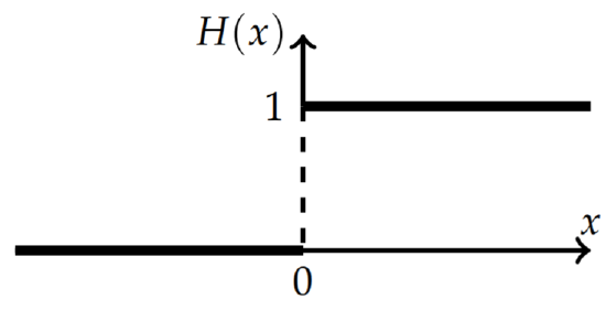
Show \(H^{\prime}(x)=\delta(x)\), where the Heaviside function (or, step function) is defined as \[H(x)= \begin{cases}0, & x<0 \\ 1, & x>0\end{cases}\nonumber \] and is shown in Figure \(\PageIndex{1}\).

Figure \(\PageIndex{1}\): The Heaviside step function, \(H(x)\).

Solution

Looking at the plot, it is easy to see that \(H^{\prime}(x)=0\) for \(x \neq 0\). In order to check that this gives the delta function, we need to compute the area integral. Therefore, we have \[\int_{-\infty}^{\infty} H^{\prime}(x) d x=\left.H(x)\right|_{-\infty} ^{\infty}=1-0=1 .\nonumber \] Thus, \(H^{\prime}(x)\) satisfies the two properties of the Dirac delta function.