10.2: The Heat Equation

Finite Difference Method

The heat equation can be solved using separation of variables. However, many partial differential equations cannot be solved exactly and one needs to turn to numerical solutions. The heat equation is a simple test case for using numerical methods. Here we will use the simplest method, finite differences.

Let us consider the heat equation in one dimension, \[u_{t}=k u_{x x} .\nonumber \] Boundary conditions and an initial condition will be applied later. The starting point is figuring out how to approximate the derivatives in this equation.

Recall that the partial derivative, \(u_{t}\), is defined by \[\frac{\partial u}{\partial t}=\lim _{\Delta t \rightarrow \infty} \frac{u(x, t+\Delta t)-u(x, t)}{\Delta t} .\nonumber \] Therefore, we can use the approximation \[\frac{\partial u}{\partial t} \approx \frac{u(x, t+\Delta t)-u(x, t)}{\Delta t} .\label{eq:1}\] This is called a forward difference approximation.

In order to find an approximation to the second derivative, \(u_{x x}\), we start with the forward difference \[\frac{\partial u}{\partial x} \approx \frac{u(x+\Delta x, t)-u(x, t)}{\Delta x} .\nonumber \] Then, \[\frac{\partial u_{x}}{\partial x} \approx \frac{u_{x}(x+\Delta x, t)-u_{x}(x, t)}{\Delta x} .\nonumber \]

We need to approximate the terms in the numerator. It is customary to use a backward difference approximation. This is given by letting \(\Delta x \rightarrow\) \(-\Delta x\) in the forward difference form, \[\frac{\partial u}{\partial x} \approx \frac{u(x, t)-u(x-\Delta x, t)}{\Delta t} .\label{eq:2}\]

Applying this to \(u_{x}\) evaluated at \(x=x\) and \(x=x+\Delta x\), we have \[u_{x}(x, t) \approx \frac{u(x, t)-u(x-\Delta x, t)}{\Delta x},\nonumber \] and \[u_{x}(x+\Delta x, t) \approx \frac{u(x+\Delta x, t)-u(x, t)}{\Delta x}\nonumber \]

Inserting these expressions into the approximation for \(u_{x x}\), we have \[\begin{align} \frac{\partial^{2} u}{\partial x^{2}} &=\frac{\partial u_{x}}{\partial x}\nonumber \\ & \approx \frac{u_{x}(x+\Delta x, t)-u_{x}(x, t)}{\Delta x}\nonumber \\ & \approx \frac{\frac{u(x+\Delta x, t)-u(x, t)}{\Delta x}}{\Delta x}-\frac{\frac{u(x, t)-u(x-\Delta x, t)}{\Delta x}}{\Delta x}\nonumber \\ &=\frac{u(x+\Delta x, t)-2 u(x, t)+u(x-\Delta x, t)}{(\Delta x)^{2}} .\label{eq:3} \end{align}\] This approximation for \(u_{x x}\) is called the central difference approximation of \(u_{x x}\).

Combining Equation \(\eqref{eq:1}\) with \(\eqref{eq:3}\) in the heat equation, we have \[\frac{u(x, t+\Delta t)-u(x, t)}{\Delta t} \approx k \frac{u(x+\Delta x, t)-2 u(x, t)+u(x-\Delta x, t)}{(\Delta x)^{2}} .\nonumber \] Solving for \(u(x, t+\Delta t)\), we find \[u(x, t+\Delta t) \approx u(x, t)+\alpha[u(x+\Delta x, t)-2 u(x, t)+u(x-\Delta x, t)],\label{eq:4}\] where \(\alpha=k \frac{\Delta t}{(\Delta x)^{2}}\).

In this equation we have a way to determine the solution at position \(x\) and time \(t+\Delta t\) given that we know the solution at three positions, \(x, x+\Delta x\), and \(x+2 \Delta x\) at time \(t\). \[u(x, t+\Delta t) \approx u(x, t)+\alpha[u(x+\Delta x, t)-2 u(x, t)+u(x-\Delta x, t)] .\label{eq:5}\]

A shorthand notation is usually used to write out finite difference schemes. The domain of the solution is \(x \in[a, b]\) and \(t \geq 0\). We seek approximate values of \(u(x, t)\) at specific positions and times. We first divide the interval \([a, b]\) into \(N\) subintervals of width \(\Delta x=(b-a) / N\). Then, the endpoints of the subintervals are given by \[x_{i}=a+i \Delta x, \quad i=0,1, \ldots, N .\nonumber \] Similarly, we take time steps of \(\Delta t\), at times \[t_{j}=j \Delta t, \quad j=0,1,2, \ldots\nonumber \] This gives a grid of points \(\left(x_{i}, t_{j}\right)\) in the domain.

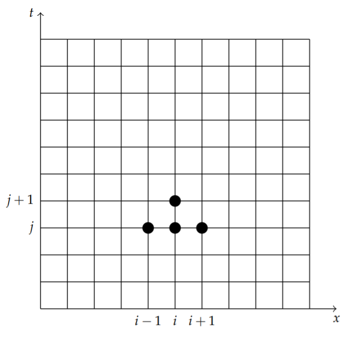
At each grid point in the domain we seek an approximate solution to the heat equation, \(u_{i, j} \approx u\left(x_{i}, t_{j}\right)\). Equation \(\eqref{eq:5}\) becomes \[u_{i, j+1} \approx u_{i, j}+\alpha\left[u_{i+1, j}-2 u_{i, j}+u_{i-1, j}\right] .\label{eq:6}\]

Equation \(\eqref{eq:7}\) is the finite difference scheme for solving the heat equation. This equation is represented by the stencil shown in Figure \(\PageIndex{1}\). The black circles represent the four terms in the equation, \(u_{i, j} u_{i-1, j} u_{i+1, j}\) and \(u_{i, j+1}\).

Figure \(\PageIndex{1}\): This stencil indicates the four types of terms in the finite difference scheme in Equation \(\eqref{eq:7}\). The black circles represent the four terms in the equation, \(u_{i, j} u_{i-1, j} u_{i+1, j}\) and \(u_{i, j+1}\).

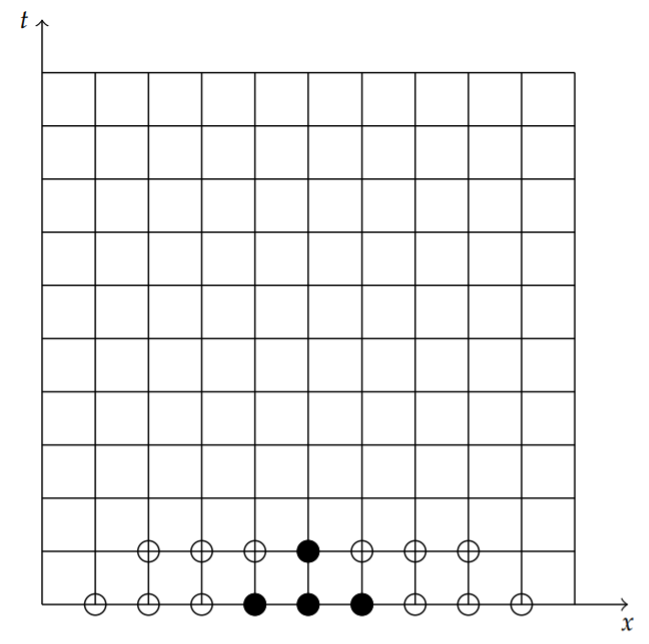
Let’s assume that the initial condition is given by \[u(x, 0)=f(x) .\nonumber \] Then, we have \(u_{i, 0}=f\left(x_{i}\right)\). Knowing these values, denoted by the open circles in Figure \(\PageIndex{2}\), we apply the stencil to generate the solution on the \(j=1\) row. This is shown in Figure \(\PageIndex{2}\).

Figure \(\PageIndex{2}\): Applying the stencil to the row of initial values gives the solution at the next time step.

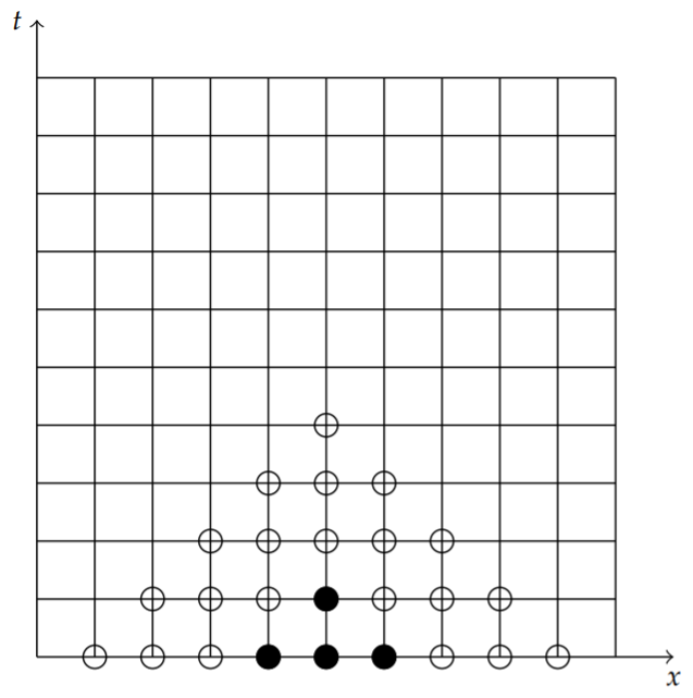
Further rows are generated by successively applying the stencil on each row, using the known approximations of \(u_{i, j}\) at each level. This gives the values of the solution at the open circles shown in Figure \(\PageIndex{3}\). We notice that the solution can only be obtained at a finite number of points on the grid.

Figure \(\PageIndex{3}\): Continuation of the process provides solutions at the indicated points.

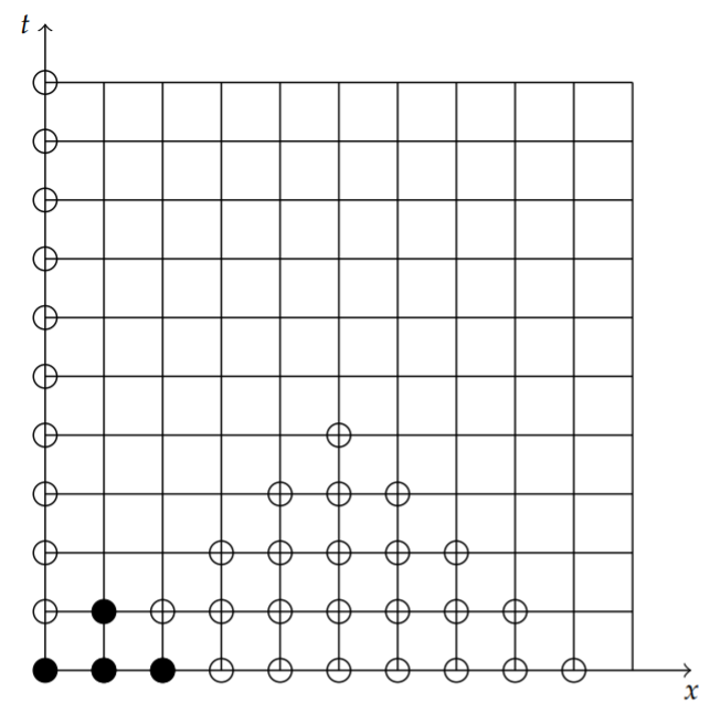
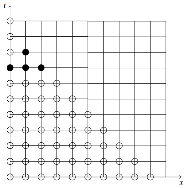
In order to obtain the missing values, we need to impose boundary conditions. For example, if we have Dirichlet conditions at \(x = a\), \[u(a, t)=0 \text {, }\nonumber \] or \(u_{0, j}=0\) for \(j=0,1, \ldots\), then we can fill in some of the missing data points as seen in Figure \(\PageIndex{4}\).

Figure \(\PageIndex{4}\): Knowing the values of the solution at \(x=a\), we can fill in more of the grid.

The process continues until we again go as far as we can. This is shown in Figure \(\PageIndex{5}\).

Figure \(\PageIndex{5}\): Knowing the values of the solution at \(x=a\), we can fill in more of the grid until we stop.

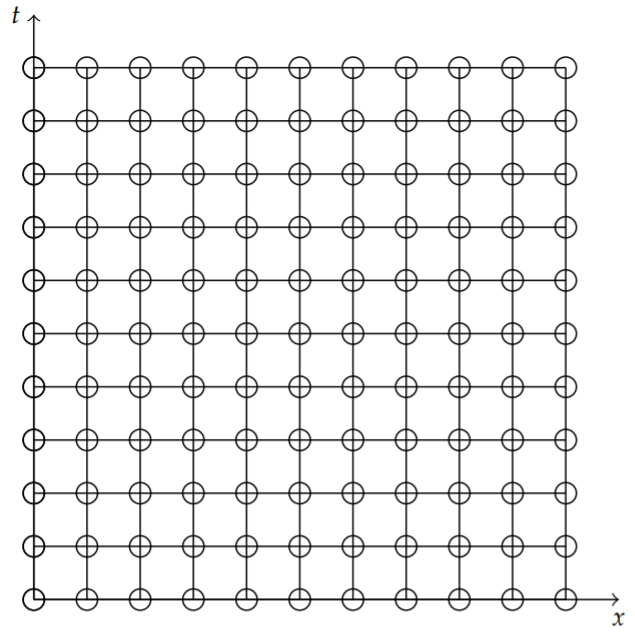
We can fill in the rest of the grid using a boundary condition at \(x=b\). For Dirichlet conditions at \(x=b\), \[u(b, t)=0,\nonumber \] or \(u_{N, j}=0\) for \(j=0,1, \ldots\), then we can fill in the rest of the missing data points as seen in Figure \(\PageIndex{6}\).

Figure \(\PageIndex{6}\): Using boundary conditions and the initial condition, the grid can be fill in through any time level.

We could also use Neumann conditions. For example, let \[u_{x}(a, t)=0 .\nonumber \] The approximation to the derivative gives \[\left.\frac{\partial u}{\partial x}\right|_{x=a} \approx \frac{u(a+\Delta x, t)-u(a, t)}{\Delta x}=0 .\nonumber \] Then, \[u(a+\Delta x, t)-u(a, t)\nonumber \] or \(u_{0, j}=u_{1, j}\), for \(j=0,1, \ldots\). Thus, we know the values at the boundary and can generate the solutions at the grid points as before.

We now have to code this using software. We can use MATLAB to do this. An example of the code is given below. In this example we specify the length of the rod, \(L=1\), and the heat constant, \(k=1\). The code is run for \(t \in[0,0.1]\).

The grid is created using \(N=10\) subintervals in space and \(M=50\) time steps. This gives \(\mathrm{dx}=\Delta x\) and \(\mathrm{dt}=\Delta t\). Using these values, we find the numerical scheme constant \(\alpha=k \Delta t /(\Delta x)^{2}\).

Nest, we define \(x_{i}=i * d x, i=0,1, \ldots, N\). However, in MATLAB, we cannot have an index of 0 . We need to start with \(i=1\). Thus, \(x_{i}=(i-1) * d x\), \(i=1,2, \ldots, N+1\).

Next, we establish the initial condition. We take a simple condition of \[u(x, 0)=\sin \pi x .\nonumber \]

We have enough information to begin the numerical scheme as developed earlier. Namely, we cycle through the time steps using the scheme. There is one loop for each time step. We will generate the new time step from the last time step in the form \[u_{i}^{\text {new }}=u_{i}^{\text {old }}+\alpha\left[u_{i+1}^{\text {old }}-2 u_{i}^{\text {old }}+u_{i-1}^{\text {old }}\right] .\label{eq:7}\] This is done using \(u 0(i)=u_{i}^{\text {new }}\) and \(u 1(i)=u_{i}^{\text {old }}\).

At the end of each time loop we update the boundary points so that the grid can be filled in as discussed. When done, we can plot the final solution. If we want to show solutions at intermediate steps, we can plot the solution earlier.

% Solution of the Heat Equation Using a Forward Difference Scheme 

% Initialize Data 
%     Length of Rod, Time Interval 
%     Number of Points in Space, Number of Time Steps 

L=1; 
T=0.1; 
k=1; 
N=10; 
M=50; 
dx=L/N; 
dt=T/M; 
alpha=k*dt/dx^2; 

% Position 

for i=1:N+1 
    x(i)=(i-1)*dx; 
end 

% Initial Condition 

for i=1:N+1 
    u0(i)=sin(pi*x(i)); 
end 

% Partial Difference Equation (Numerical Scheme) 

for j=1:M 
    for i=2:N 
        u1(i)=u0(i)+alpha*(u0(i+1)-2*u0(i)+u0(i-1)); 
    end 
    u1(1)=0; 
    u1(N+1)=0; 
    u0=u1; 
end 

% Plot solution 
plot(x, u1);