
11.5: Integrals
- Page ID
- 91029

Integration is typically a bit harder. Imagine being given the last result in (11.4.2) and having to figure out what was differentiated in order to get the given function. As you may recall from the Fundamental Theorem of Calculus, the integral is the inverse operation to differentiation: \[\int \frac{d f}{d x} d x=f(x)+C .\label{eq:1}\]
It is not always easy to evaluate a given integral. In fact some integrals are not even doable! However, you learned in calculus that there are some methods that could yield an answer. While you might be happier using a computer algebra system, such as Maple or WolframAlpha.com, or a fancy calculator, you should know a few basic integrals and know how to use tables for some of the more complicated ones. In fact, it can be exhilarating when you can do a given integral without reference to a computer or a Table of Integrals. However, you should be prepared to do some integrals using what you have been taught in calculus. We will review a few of these methods and some of the standard integrals in this section.
First of all, there are some integrals you are expected to know without doing any work. These integrals appear often and are just an application of the Fundamental Theorem of Calculus to the previous Table 11.4.1. The basic integrals that students should know off the top of their heads are given in Table \(\PageIndex{1}\).
These are not the only integrals you should be able to do. We can expand the list by recalling a few of the techniques that you learned in calculus, the Method of Substitution, Integration by Parts, integration using partial fraction decomposition, and trigonometric integrals, and trigonometric substitution. There are also a few other techniques that you had not seen before. We will look at several examples.
Evaluate \(\int \frac{x}{\sqrt{x^{2}+1}} d x\).
Solution
When confronted with an integral, you should first ask if a simple substitution would reduce the integral to one you know how to do.
The ugly part of this integral is the \(x^{2}+1\) under the square root. So, we let \(u=x^{2}+1\).
Noting that when \(u=f(x)\), we have \(d u=f^{\prime}(x) d x\). For our example, \(d u=\) \(2 x d x\).
Looking at the integral, part of the integrand can be written as \(x d x=\frac{1}{2} u d u\). Then, the integral becomes \[\int \frac{x}{\sqrt{x^{2}+1}} d x=\frac{1}{2} \int \frac{d u}{\sqrt{u}} .\nonumber \]
The substitution has converted our integral into an integral over \(u\). Also, this integral is doable! It is one of the integrals we should know. Namely, we can write it as \[\frac{1}{2} \int \frac{d u}{\sqrt{u}}=\frac{1}{2} \int u^{-1 / 2} d u .\nonumber \] This is now easily finished after integrating and using the substitution variable to give \[\int \frac{x}{\sqrt{x^{2}+1}} d x=\frac{1}{2} \frac{u^{1 / 2}}{\frac{1}{2}}+C=\sqrt{x^{2}+1}+C .\nonumber \] Note that we have added the required integration constant and that the derivative of the result easily gives the original integrand (after employing the Chain Rule).
Table \(\PageIndex{1}\): Table of Common Integrals.
| Function | Indefinite Integral |
|---|---|
| \(a\) | \(a x\) |
| \(x^{n}\) | \(\frac{x^{n+1}}{n+1}\) |
| \(e^{a x}\) | \(\frac{1}{a} e^{a x}\) |
| \(\frac{1}{x}\) | \(\ln x\) |
| \(\sin a x\) | \(-\frac{1}{a} \cos a x\) |
| \(\cos a x\) | \(\frac{1}{a} \sin a x\) |
| \(\sec ^{2} a x\) | \(\frac{1}{a} \tan a x\) |
| \(\sinh a x\) | \(\frac{1}{a} \cosh a x\) |
| \(\cosh a x\) | \(\frac{1}{a} \sinh a x\) |
| \(\operatorname{sech}^{2} a x\) | \(\frac{1}{a} \tanh a x\) |
| \(\sec x\) | \(\ln |\sec x+\tan x|\) |
| \(\frac{1}{a+b x}\) | \(\frac{1}{b} \ln (a+b x)\) |
| \(\frac{1}{a^{2}+x^{2}}\) | \(\frac{1}{a} \tan ^{-1} \frac{x}{a}\) |
| \(\frac{1}{\sqrt{a^{2}-x^{2}}}\) | \(\sin ^{-1} \frac{x}{a}\) |
| \(\frac{1}{x \sqrt{x^{2}-a^{2}}}\) | \(\frac{1}{a} \sec ^{-1} \frac{x}{a}\) |
| \(\frac{1}{\sqrt{x^{2}-a^{2}}}\) | \(\cosh ^{-1} \frac{x}{a}=\ln \left|\sqrt{x^{2}-a^{2}}+x\right|\) |
Often we are faced with definite integrals, in which we integrate between two limits. There are several ways to use these limits. However, students often forget that a change of variables generally means that the limits have to change.
Evaluate \(\int_{0}^{2} \frac{x}{\sqrt{x^{2}+1}} d x\).
Solution
This is the last example but with integration limits added. We proceed as before. We let \(u=x^{2}+1\). As \(x\) goes from \(0\) to \(2,\: u\) takes values from \(1\) to \(5\). So, this substitution gives \[\int_{0}^{2} \frac{x}{\sqrt{x^{2}+1}} d x=\frac{1}{2} \int_{1}^{5} \frac{d u}{\sqrt{u}}=\left.\sqrt{u}\right|_{1} ^{5}=\sqrt{5}-1 .\nonumber \]
When you becomes proficient at integration, you can bypass some of these steps. In the next example we try to demonstrate the thought process involved in using substitution without explicitly using the substitution variable. Example \(\PageIndex{3}\).
Evaluate \(\int_{0}^{2} \frac{x}{\sqrt{9+4 x^{2}}} d x\)
Solution
As with the previous example, one sees that the derivative of \(9+4 x^{2}\) is proportional to \(x\), which is in the numerator of the integrand. Thus a substitution would give an integrand of the form \(u^{-1 / 2}\). So, we expect the answer to be proportional to \(\sqrt{u}=\sqrt{9+4 x^{2}}\). The starting point is therefore, \[\int \frac{x}{\sqrt{9+4 x^{2}}} d x=A \sqrt{9+4 x^{2}},\nonumber \] where \(A\) is a constant to be determined.
We can determine \(A\) through differentiation since the derivative of the answer should be the integrand. Thus, \[\begin{align} \frac{d}{d x} A\left(9+4 x^{2}\right)^{\frac{1}{2}} &=A\left(9+4 x^{2}\right)^{-\frac{1}{2}}\left(\frac{1}{2}\right)(8 x)\nonumber \\ &=4 x A\left(9+4 x^{2}\right)^{-\frac{1}{2}}\label{eq:2} \end{align}\] Comparing this result with the integrand, we see that the integrand is obtained when \(A=\frac{1}{4}\). Therefore, \[\int \frac{x}{\sqrt{9+4 x^{2}}} d x=\frac{1}{4} \sqrt{9+4 x^{2}} .\nonumber \]
We now complete the integral, \[\int_{0}^{2} \frac{x}{\sqrt{9+4 x^{2}}} d x=\frac{1}{4}[5-3]=\frac{1}{2} .\nonumber \]
The function \[\operatorname{gd}(x)=\int_{0}^{x} \frac{d x}{\cosh x}=2 \tan ^{-1} e^{x}-\frac{\pi}{2}\nonumber\] is called the Gudermannian and connects trigonometric and hyperbolic functions. This function was named after Christoph Gudermann ( \(1798-1852\) ), but introduced by Iohann Heinrich Lambert ( \(1728-1777\) ), who was one of the first to introduce hyperbolic functions.
Evaluate \(\int \frac{d x}{\cosh x}\).
Solution
This integral can be performed by first using the definition of \(\cosh x\) followed by a simple substitution. \[\begin{align} \int \frac{d x}{\cosh x} &=\int \frac{2}{e^{x}+e^{-x}} d x\nonumber \\ &=\int \frac{2 e^{x}}{e^{2 x}+1} d x .\label{eq:3} \end{align}\]
Now, we let \(u=e^{x}\) and \(d u=e^{x} d x\). Then, \[\begin{align} \int \frac{d x}{\cosh x} &=\int \frac{2}{1+u^{2}} d u\nonumber \\ &=2 \tan ^{-1} u+C\nonumber \\ &=2 \tan ^{-1} e^{x}+C .\label{eq:4} \end{align}\]
11.5.1 Integration by Parts
When the Method of Substitution fails, there are other methods you can try. One of the most used is the Method of Integration by Parts. Recall the Integration by Parts Formula: \[\int u d v=u v-\int v d u \label{eq:5}\] The idea is that you are given the integral on the left and you can relate it to an integral on the right. Hopefully, the new integral is one you can do, or at least it is an easier integral than the one you are trying to evaluate.
However, you are not usually given the functions \(u\) and \(v\). You have to determine them. The integral form that you really have is a function of another variable, say \(x\). Another form of the Integration by Parts Formula can be written as \[\int f(x) g^{\prime}(x) d x=f(x) g(x)-\int g(x) f^{\prime}(x) d x .\label{eq:6}\] This form is a bit more complicated in appearance, though it is clearer than the \(u-v\) form as to what is happening. The derivative has been moved from one function to the other. Recall that this formula was derived by integrating the product rule for differentiation. (See your calculus text.)
Often in physics one needs to move a derivative between functions inside an integrand. The key - use integration by parts to move the derivative from one function to the other under an integral.
These two formulae can be related by using the differential relations \[\begin{align} &u=f(x) \quad \rightarrow \quad d u=f^{\prime}(x) d x\nonumber \\ &v=g(x) \quad \rightarrow \quad d v=g^{\prime}(x) d x .\label{eq:7} \end{align}\] This also gives a method for applying the Integration by Parts Formula.
Consider the integral \(\int x \sin 2 x d x\).
Solution
We choose \(u=x\) and \(d v=\) \(\sin 2 x d x\). This gives the correct left side of the Integration by Parts Formula. We next determine \(v\) and \(d u\) : \[\begin{gathered} d u=\frac{d u}{d x} d x=d x, \\ v=\int d v=\int \sin 2 x d x=-\frac{1}{2} \cos 2 x . \end{gathered}\] We note that one usually does not need the integration constant. Inserting these expressions into the Integration by Parts Formula, we have \[\int x \sin 2 x d x=-\frac{1}{2} x \cos 2 x+\frac{1}{2} \int \cos 2 x d x .\nonumber \] We see that the new integral is easier to do than the original integral. Had we picked \(u=\sin 2 x\) and \(d v=x d x\), then the formula still works, but the resulting integral is not easier.
For completeness, we finish the integration. The result is \[\int x \sin 2 x d x=-\frac{1}{2} x \cos 2 x+\frac{1}{4} \sin 2 x+C \text {. }\nonumber \]
As always, you can check your answer by differentiating the result, a step students often forget to do. Namely, \[\begin{align}\frac{d}{d x}\left(-\frac{1}{2} x \cos 2 x+\frac{1}{4} \sin 2 x+C\right)&=-\frac{1}{2} \cos 2 x+x \sin 2 x+\frac{1}{4}(2 \cos 2 x)\nonumber \\ &=x \sin 2 x \text {. }\label{eq:8}\end{align}\] So, we do get back the integrand in the original integral.
We can also perform integration by parts on definite integrals. The general formula is written as \[\int_{a}^{b} f(x) g^{\prime}(x) d x=\left.f(x) g(x)\right|_{a} ^{b}-\int_{a}^{b} g(x) f^{\prime}(x) d x \text {. }\label{eq:9}\]
Consider the integral \[\int_{0}^{\pi} x^{2} \cos x d x.\nonumber \]
Solution
This will require two integrations by parts. First, we let \(u=x^{2}\) and \(d v=\cos x\). \[d u=2 x d x . \quad v=\sin x\nonumber \] Inserting into the Integration by Parts Formula, we have \[\begin{align} \int_{0}^{\pi} x^{2} \cos x d x &=\left.x^{2} \sin x\right|_{0} ^{\pi}-2 \int_{0}^{\pi} x \sin x d x\nonumber \\ &=-2 \int_{0}^{\pi} x \sin x d x .\label{eq:10} \end{align}\]
We note that the resulting integral is easier that the given integral, but we still cannot do the integral off the top of our head (unless we look at Example 3!). So, we need to integrate by parts again. (Note: In your calculus class you may recall that there is a tabular method for carrying out multiple applications of the formula. We will show this method in the next example.)
We apply integration by parts by letting \(U=x\) and \(d V=\sin x d x\). This gives \(d U=d x\) and \(V=-\cos x\). Therefore, we have \[\begin{align} \int_{0}^{\pi} x \sin x d x &=-\left.x \cos x\right|_{0} ^{\pi}+\int_{0}^{\pi} \cos x d x\nonumber \\ &=\pi+\left.\sin x\right|_{0} ^{\pi}\nonumber \\ &=\pi .\label{eq:11} \end{align}\]
The final result is \[\int_{0}^{\pi} x^{2} \cos x d x=-2 \pi \text {. }\nonumber \]
There are other ways to compute integrals of this type. First of all, there is the Tabular Method to perform integration by parts. A second method is to use differentiation of parameters under the integral. We will demonstrate this using examples.
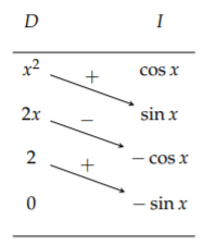
Compute the integral \(\int_{0}^{\pi} x^{2} \cos x d x\) using the Tabular Method.
Solution
First we identify the two functions under the integral, \(x^{2}\) and \(\cos x\). We then write the two functions and list the derivatives and integrals of each, respectively. This is shown in Table \(\PageIndex{2}\). Note that we stopped when we reached zero in the left column.
Next, one draws diagonal arrows, as indicated, with alternating signs attached, starting with \(+\). The indefinite integral is then obtained by summing the products of the functions at the ends of the arrows along with the signs on each arrow: \[\int x^{2} \cos x d x=x^{2} \sin x+2 x \cos x-2 \sin x+C .\nonumber \] To find the definite integral, one evaluates the antiderivative at the given limits. \[\begin{align} \int_{0}^{\pi} x^{2} \cos x d x &=\left[x^{2} \sin x+2 x \cos x-2 \sin x\right]_{0}^{\pi}\nonumber \\ &=\left(\pi^{2} \sin \pi+2 \pi \cos \pi-2 \sin \pi\right)-0\nonumber \\ &=-2 \pi .\label{eq:12} \end{align}\]
Actually, the Tabular Method works even if a zero does not appear in the left column. One can go as far as possible, and if a zero does not appear, then one needs only integrate, if possible, the product of the functions in the last row, adding the next sign in the alternating sign progression. The next example shows how this works.
Table \(\PageIndex{2}\): Tabular Method
Use the Tabular Method to compute \(\int e^{2 x} \sin 3 x d x\).
Solution
As before, we first set up the table as shown in Table \(\PageIndex{3}\).
Table \(\PageIndex{3}\): Tabular Method, showing a nonterminating example.
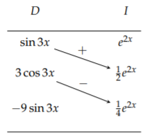
Putting together the pieces, noting that the derivatives in the left column will never vanish, we have \[\int e^{2 x} \sin 3 x d x=\left(\frac{1}{2} \sin 3 x-\frac{3}{4} \cos 3 x\right) e^{2 x}+\int(-9 \sin 3 x)\left(\frac{1}{4} e^{2 x}\right) d x.\nonumber\] The integral on the right is a multiple of the one on the left, so we can combine them, \[\frac{13}{4} \int e^{2 x} \sin 3 x d x=\left(\frac{1}{2} \sin 3 x-\frac{3}{4} \cos 3 x\right) e^{2 x},\nonumber \] or \[\int e^{2 x} \sin 3 x d x=\left(\frac{2}{13} \sin 3 x-\frac{3}{13} \cos 3 x\right) e^{2 x} .\nonumber \]
11.5.2 Differentiation Under the Integral
Another method that one can use to evaluate this integral is to differentiate under the integral sign. This is mentioned in the Richard Feynman’s memoir Surely You’re Joking, Mr. Feynman!. In the book Feynman recounts using this "trick" to be able to do integrals that his MIT classmates could not do. This is based on a theorem found in Advanced Calculus texts. Reader’s unfamiliar with partial derivatives should be able to grasp their use in the following example.
Let the functions \(f(x, t)\) and \(\frac{\partial f(x, t)}{\partial x}\) be continuous in both \(t\), and \(x\), in the region of the \((t, x)\) plane which includes \(a(x) \leq t \leq b(x), x_{0} \leq x \leq x_{1}\), where the functions \(a(x)\) and \(b(x)\) are continuous and have continuous derivatives for \(x_{0} \leq x \leq x_{1}\). Defining \[F(x) \equiv \int_{a(x)}^{b(x)} f(x, t) d t,\nonumber \] then \[\begin{align} \frac{d F(x)}{d x} &=\left(\frac{\partial F}{\partial b}\right) \frac{d b}{d x}+\left(\frac{\partial F}{\partial a}\right) \frac{d a}{d x}+\int_{a(x)}^{b(x)} \frac{\partial}{\partial x} f(x, t) d t\nonumber \\ &=f(x, b(x)) b^{\prime}(x)-f(x, a(x)) a^{\prime}(x)+\int_{a(x)}^{b(x)} \frac{\partial}{\partial x} f(x, t) d t.\label{eq:13} \end{align}\] for \(x_{0} \leq x \leq x_{1}\). This is a generalized version of the Fundamental Theorem of Calculus.
In the next examples we show how we can use this theorem to bypass integration by parts.
Use differentiation under the integral sign to evaluate \(\int x e^{x} d x\).
Solution
First, consider the integral \[I(x, a)=\int e^{a x} d x=\frac{e^{a x}}{a} .\nonumber \] Then, \[\frac{\partial I(x, a)}{\partial a}=\int x e^{a x} d x\nonumber \] So, \[\begin{align} \int x e^{a x} d x &=\frac{\partial I(x, a)}{\partial a}\nonumber \\ &=\frac{\partial}{\partial a}\left(\int e^{a x} d x\right)\nonumber \\ &=\frac{\partial}{\partial a}\left(\frac{e^{a x}}{a}\right)\nonumber \\ &=\left(\frac{x}{a}-\frac{1}{a^{2}}\right) e^{a x}\label{eq:14} \end{align}\] Evaluating this result at \(a=1\), we have \[\int x e^{x} d x=(x-1) e^{x} .\nonumber \]
The reader can verify this result by employing the previous methods or by just differentiating the result.
We will do the integral \(\int_{0}^{\pi} x^{2} \cos x d x\) once more.
Solution
First, consider the integral \[\begin{align} I(a) & \equiv \int_{0}^{\pi} \cos a x d x\nonumber \\ &=\left.\frac{\sin a x}{a}\right|_{0} ^{\pi}\nonumber \\ &=\frac{\sin a \pi}{a} .\label{eq:15} \end{align}\] Differentiating the integral \(I(a)\) with respect to a twice gives \[\frac{d^{2} I(a)}{d a^{2}}=-\int_{0}^{\pi} x^{2} \cos a x d x .\label{eq:16}\] Evaluation of this result at \(a=1\) leads to the desired result. Namely, \[\begin{align} \int_{0}^{\pi} x^{2} \cos x d x &=-\left.\frac{d^{2} I(a)}{d a^{2}}\right|_{a=1}\nonumber \\ &=-\left.\frac{d^{2}}{d a^{2}}\left(\frac{\sin a \pi}{a}\right)\right|_{a=1}\nonumber \\ &=-\left.\frac{d}{d a}\left(\frac{a \pi \cos a \pi-\sin a \pi}{a^{2}}\right)\right|_{a=1}\nonumber \\ &=-\left.\left(\frac{a^{2} \pi^{2} \sin a \pi+2 a \pi \cos a \pi-2 \sin a \pi}{a^{3}}\right)\right|_{a=1}\nonumber \\ &=-2 \pi .\label{eq:17} \end{align}\]
11.5.3 Trigonometric Integrals
Other types of integrals that you will see often are trigonometric integrals. In particular, integrals involving powers of sines and cosines. For odd powers, a simple substitution will turn the integrals into simple powers.
For example, consider \[\int \cos ^{3} x d x.\nonumber \]
Solution
This can be rewritten as \[\int \cos ^{3} x d x=\int \cos ^{2} x \cos x d x.\nonumber \] Let \(u=\sin x\). Then, \(d u=\cos x d x\). Since \(\cos ^{2} x=1-\sin ^{2} x\), we have \[\begin{align} \int \cos ^{3} x d x &=\int \cos ^{2} x \cos x d x\nonumber \\ &=\int\left(1-u^{2}\right) d u\nonumber \\ &=u-\frac{1}{3} u^{3}+C\nonumber \\ &=\sin x-\frac{1}{3} \sin ^{3} x+C.\label{eq:18} \end{align}\] A quick check confirms the answer: \[\begin{align} \frac{d}{d x}\left(\sin x-\frac{1}{3} \sin ^{3} x+C\right) &=\cos x-\sin ^{2} x \cos x\nonumber \\ &=\cos x\left(1-\sin ^{2} x\right)\nonumber \\ &=\cos ^{3} x .\label{eq:19} \end{align}\]
Even powers of sines and cosines are a little more complicated, but doable. In these cases we need the half angle formulae (11.2.12)-(11.2.13).
As an example, we will compute \[\int_{0}^{2 \pi} \cos ^{2} x d x \text {. }\nonumber\]
Solution
Substituting the half angle formula for \(\cos ^{2} x\), we have \[\begin{align} \int_{0}^{2 \pi} \cos ^{2} x d x &=\frac{1}{2} \int_{0}^{2 \pi}(1+\cos 2 x) d x\nonumber \\ &=\frac{1}{2}\left(x-\frac{1}{2} \sin 2 x\right)_{0}^{2 \pi}\nonumber \\ &=\pi\label{eq:20} \end{align}\]
Recall that RMS averages refer to the root mean square average. This is computed by first computing the average, or mean, of the square of some quantity. Then one takes the square root. Typical examples are RMS voltage, RMS current, and the average energy in an electromagnetic wave. AC currents oscillate so fast that the measured value is the RMS voltage.
We note that this result appears often in physics. When looking at root mean square averages of sinusoidal waves, one needs the average of the square of sines and cosines. Recall that the average of a function on interval \([a, b]\) is given as \[f \text { ave }=\frac{1}{b-a} \int_{a}^{b} f(x) d x.\label{eq:21}\] So, the average of \(\cos ^{2} x\) over one period is \[\frac{1}{2 \pi} \int_{0}^{2 \pi} \cos ^{2} x d x=\frac{1}{2} \text {. }\label{eq:22}\] The root mean square is then found by taking the square root, \(\frac{1}{\sqrt{2}}\).
11.5.4 Trigonometric Function Substitution
Another class of integrals typically studied in calculus are those involving the forms \(\sqrt{1-x^{2}}, \sqrt{1+x^{2}}\), or \(\sqrt{x^{2}-1}\). These can be simplified through the use of trigonometric substitutions. The idea is to combine the two terms under the radical into one term using trigonometric identities. We will consider some typical examples.
Evaluate \(\int \sqrt{1-x^{2}} d x\).
Solution
Since \(1-\sin ^{2} \theta=\cos ^{2} \theta\), we perform the sine substitution \[x=\sin \theta, \quad d x=\cos \theta d \theta .\nonumber \] Then, \[\begin{align} \int \sqrt{1-x^{2}} d x &=\int \sqrt{1-\sin ^{2} \theta} \cos \theta d \theta\nonumber \\ &=\int \cos ^{2} \theta d \theta .\label{eq:23} \end{align}\] Using the last example, we have \[\int \sqrt{1-x^{2}} d x=\frac{1}{2}\left(\theta-\frac{1}{2} \sin 2 \theta\right)+C .\nonumber \]
However, we need to write the answer in terms of \(x\). We do this by first using the double angle formula for \(\sin 2 \theta\) and \(\cos \theta=\sqrt{1-x^{2}}\) to obtain \[\int \sqrt{1-x^{2}} d x=\frac{1}{2}\left(\sin ^{-1} x-x \sqrt{1-x^{2}}\right)+C .\nonumber \]
In any of these computations careful attention has to be paid to simplifying the radical. This is because \[\sqrt{x^{2}}=|x| \text {. }\nonumber \] For example, \(\sqrt{(-5)^{2}}=\sqrt{25}=5\). For \(x=\sin \theta\), one typically specifies the domain \(-\pi / 2 \leq \theta \leq \pi / 2\). In this domain we have \(|\cos \theta|=\cos \theta\).
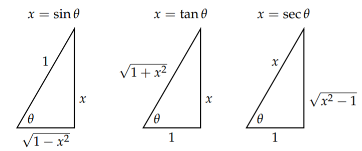
Similar trigonometric substitutions result for integrands involving \(\sqrt{1+x^{2}}\) and \(\sqrt{x^{2}-1}\). The substitutions are summarized in Table \(\PageIndex{4}\). The simplification of the given form is then obtained using trigonometric identities. This can also be accomplished by referring to the right triangles shown in Figure \(\PageIndex{1}\).
Table \(\PageIndex{4}\): Standard trigonometric substitutions.
| Form | Substitution | Differential |
|---|---|---|
| \(\sqrt{a^{2}-x^{2}}\) | \(x=a \sin \theta\) | \(d x=a \cos \theta d \theta\) |
| \(\sqrt{a^{2}+x^{2}}\) | \(x=a \tan \theta\) | \(d x=a \sec ^{2} \theta d \theta\) |
| \(\sqrt{x^{2}-a^{2}}\) | \(x=a \sec \theta\) | \(d x=a \sec \theta \tan \theta d \theta\) |
Evaluate \(\int_{0}^{2} \sqrt{x^{2}+4} d x\).
Solution
Let \(x=2 \tan \theta\). Then, \(d x=2 \sec ^{2} \theta d \theta\) and \[\sqrt{x^2+4}=\sqrt{4\tan^2\theta +4}=2\sec\theta.\nonumber\] So, the integral becomes \[\int_{0}^{2} \sqrt{x^{2}+4} d x=4 \int_{0}^{\pi / 4} \sec ^{3} \theta d \theta\nonumber \]
One has to recall, or look up, \[\int \sec ^{3} \theta d \theta=\frac{1}{2}(\tan \theta \sec \theta+\ln |\sec \theta+\tan \theta|)+C .\nonumber \] This gives \[\begin{align} \int_{0}^{2} \sqrt{x^{2}+4} d x &=2[\tan \theta \sec \theta+\ln |\sec \theta+\tan \theta|]_{0}^{\pi / 4}\nonumber \\ &=2(\sqrt{2}+\ln |\sqrt{2}+1|-(0+\ln (1)))\nonumber \\ &=2(\sqrt{2}+\ln (\sqrt{2}+1)) .\label{eq:24} \end{align}\]
Evaluate \(\int \frac{d x}{\sqrt{x^{2}-1}}, x \geq 1\).
Solution
In this case one needs the secant substitution. This yields \[\begin{align} \int \frac{d x}{\sqrt{x^{2}-1}} &=\int \frac{\sec \theta \tan \theta d \theta}{\sqrt{\sec ^{2} \theta-1}}\nonumber \\ &=\int \frac{\sec \theta \tan \theta d \theta}{\tan \theta}\nonumber \\ &=\int \sec \theta d \theta\nonumber \\ &=\ln (\sec \theta+\tan \theta)+C\nonumber \\ &=\ln \left(x+\sqrt{x^{2}-1}\right)+C .\label{eq:25} \end{align}\]
Evaluate \(\int \frac{d x}{x \sqrt{x^{2}-1}}, x \geq 1\)
Solution
Again we can use a secant substitution. This yields \[\begin{align} \int \frac{d x}{x \sqrt{x^{2}-1}} &=\int \frac{\sec \theta \tan \theta d \theta}{\sec \theta \sqrt{\sec ^{2} \theta-1}}\nonumber \\ &=\int \frac{\sec \theta \tan \theta}{\sec \theta \tan \theta} d \theta\nonumber \\ &=\int d \theta=\theta+C=\sec ^{-1} x+C .\label{eq:26} \end{align}\]
11.5.5 Hyperbolic Function Substitution
Even though trigonometric substitution plays a role in the calculus program, students often see hyperbolic function substitution used in physics courses. The reason might be because hyperbolic function substitution is sometimes simpler. The idea is the same as for trigonometric substitution. We use an identity to simplify the radical.
Evaluate \(\int_{0}^{2} \sqrt{x^{2}+4} d x\) using the substitution \(x=2 \sinh u\).
Solution
Since \(x=2 \sinh u\), we have \(d x=2 \cosh u d u\). Also, we can use the identity \(\cosh ^{2} u-\sinh ^{2} u=1\) to rewrite \[\sqrt{x^{2}+4}=\sqrt{4 \sinh ^{2} u+4}=2 \cosh u \text {. }\nonumber \]
The integral can be now be evaluated using these substitutions and some hyperbolic function identities, \[\begin{align} \int_{0}^{2} \sqrt{x^{2}+4} d x&=4 \int_{0}^{\sinh ^{-1} 1} \cosh ^{2} u d u\nonumber \\ &=2 \int_{0}^{\sinh ^{-1} 1}(1+\cosh 2 u) d u\nonumber \\ &=2\left[u+\frac{1}{2} \sinh 2 u\right]_{0}^{\sinh ^{-1} 1}\nonumber \\ &=2[u+\sinh u \cosh u]_{0}^{\sinh ^{-1} 1}\nonumber \\ &=2\left(\sinh ^{-1} 1+\sqrt{2}\right) .\label{eq:27} \end{align}\]
In Example \(\PageIndex{14}\) we used a trigonometric substitution and found \[\int_{0}^{2} \sqrt{x^{2}+4}=2(\sqrt{2}+\ln (\sqrt{2}+1)) .\nonumber \] This is the same result since \(\sinh ^{-1} 1=\ln (1+\sqrt{2})\).
Evaluate \(\int \frac{d x}{\sqrt{x^{2}-1}}\) for \(x \geq 1\) using hyperbolic function substitution.
Solution
This integral was evaluated in Example \(\PageIndex{16}\) using the trigonometric substitution \(x=\sec \theta\) and the resulting integral of \(\sec \theta\) had to be recalled. Here we will use the substitution \[x=\cosh u, \quad d x=\sinh u d u, \quad \sqrt{x^{2}-1}=\sqrt{\cosh ^{2} u-1}=\sinh u .\nonumber \]
Then, \[\begin{align} \int \frac{d x}{\sqrt{x^{2}-1}} &=\int \frac{\sinh u d u}{\sinh u}\nonumber \\ &=\int d u=u+C\nonumber \\ &=\cosh ^{-1} x+C\nonumber \\ &=\frac{1}{2} \ln \left(x+\sqrt{x^{2}-1}\right)+C,\label{eq:28} \quad x \geq 1 \end{align}\]
This is the same result as we had obtained previously, but this derivation was a little cleaner.
Also, we can extend this result to values \(x \leq-1\) by letting \(x=-\cosh u\). This gives \[\int \frac{d x}{\sqrt{x^{2}-1}}=\frac{1}{2} \ln \left(x+\sqrt{x^{2}-1}\right)+C, \quad x \leq-1 .\nonumber \]
Combining these results, we have shown \[\int \frac{d x}{\sqrt{x^{2}-1}}=\frac{1}{2} \ln \left(|x|+\sqrt{x^{2}-1}\right)+C, \quad x^{2} \geq 1 .\nonumber \]
We have seen in the last example that the use of hyperbolic function substitution allows us to bypass integrating the secant function in Example \(\PageIndex{16}\) when using trigonometric substitutions. In fact, we can use hyperbolic substitutions to evaluate integrals of powers of secants. Comparing Examples \(\PageIndex{16}\) and \(\PageIndex{18}\), we consider the transformation \(\sec \theta=\cosh u\). The relation between differentials is found by differentiation, giving \[\sec \theta \tan \theta d \theta=\sinh u d u\nonumber \] Since \[\tanh ^{2} \theta=\sec ^{2} \theta-1,\nonumber \] we have \(\tan \theta=\sinh u\), therefore \[d \theta=\frac{d u}{\cosh u} .\nonumber \] In the next example we show how useful this transformation is.
Evaluate \(\int \sec \theta d \theta\) using hyperbolic function substitution.
Solution
From the discussion in the last paragraph, we have \[\begin{align} \int \sec \theta d \theta &=\int d u\nonumber \\ &=u+C\nonumber \\ &=\cosh ^{-1}(\sec \theta)+C\label{eq:29} \end{align}\]
We can express this result in the usual form by using the logarithmic form of the inverse hyperbolic cosine, \[\cosh ^{-1} x=\ln \left(x+\sqrt{x^{2}-1}\right) \text {. }\nonumber \] The result is \[\int \sec \theta d \theta=\ln (\sec \theta+\tan \theta) .\nonumber \]
This example was fairly simple using the transformation \(\sec \theta=\cosh u\). Another common integral that arises often is integrations of \(\sec ^{3} \theta\). In a typical calculus class this integral is evaluated using integration by parts. However. that leads to a tricky manipulation that is a bit scary the first time it is encountered (and probably upon several more encounters.) In the next example, we will show how hyperbolic function substitution is simpler.
Evaluate \(\int \sec ^{3} \theta d \theta\) using hyperbolic function substitution.
Solution
First, we consider the transformation \(\sec \theta=\cosh u\) with \(d \theta=\frac{d u}{\cosh u}\). Then, \[\int \sec ^{3} \theta d \theta=\int \frac{d u}{\cosh u} .\nonumber \] This integral was done in Example \(\PageIndex{4}\), leading to \[\int \sec ^{3} \theta d \theta=2 \tan ^{-1} e^{u}+C .\nonumber \]
While correct, this is not the form usually encountered. Instead, we make the slightly different transformation \(\tan \theta=\sinh u\). Since \(\sec ^{2} \theta=1+\tan ^{2} \theta\), we find \(\sec \theta=\cosh u\). As before, we find \[d \theta=\frac{d u}{\cosh u} .\nonumber \] Using this transformation and several identities, the integral becomes \[\begin{align}\int \sec ^{3} \theta d \theta &=\int \cosh ^{2} u d u\nonumber \\ &=\frac{1}{2} \int(1+\cosh 2 u) d u\nonumber \\ &=\frac{1}{2}\left(u+\frac{1}{2} \sinh 2 u\right)\nonumber \\ &=\frac{1}{2}(u+\sinh u \cosh u)\nonumber \\ &=\frac{1}{2}\left(\cosh ^{-1}(\sec \theta)+\tan \theta \sec \theta\right)\nonumber \\ &=\frac{1}{2}(\sec \theta \tan \theta+\ln (\sec \theta+\tan \theta)) .\label{eq:30} \end{align}\]
There are many other integration methods, some of which we will visit in other parts of the book, such as partial fraction decomposition and numerical integration. Another topic which we will revisit is power series.