12.1: First Order Differential Equations

Before moving on, we first define an \(n\)-th order ordinary differential equation. It is an equation for an unknown function \(y(x)\) that expresses a relationship between the unknown function and its first \(n\) derivatives. One could write this generally as \[F\left(y^{(n)}(x), y^{(n-1)}(x), \ldots, y^{\prime}(x), y(x), x\right)=0 .\label{eq:1}\] Here \(y^{(n)}(x)\) represents the \(n\)th derivative of \(y(x)\).

An initial value problem consists of the differential equation plus the values of the first \(n-1\) derivatives at a particular value of the independent variable, say \(x_{0}\) : \[y^{(n-1)}\left(x_{0}\right)=y_{n-1}, \quad y^{(n-2)}\left(x_{0}\right)=y_{n-2}, \quad \ldots, \quad y\left(x_{0}\right)=y_{0} .\label{eq:2}\]

A linear \(n\)th order differential equation takes the form \[\left.a_{n}(x) y^{(n)}(x)+a_{n-1}(x) y^{(n-1)}(x)+\ldots+a_{1}(x) y^{\prime}(x)+a_{0}(x) y(x)\right)=f(x) .\label{eq:3}\] If \(f(x) \equiv 0\), then the equation is said to be homogeneous, otherwise it is called nonhomogeneous.

Typically, the first differential equations encountered are first order equations. A first order differential equation takes the form \[F\left(y^{\prime}, y, x\right)=0 .\label{eq:4} \] There are two common first order differential equations for which one can formally obtain a solution. The first is the separable case and the second is a first order equation. We indicate that we can formally obtain solutions, as one can display the needed integration that leads to a solution. However, the resulting integrals are not always reducible to elementary functions nor does one obtain explicit solutions when the integrals are doable.

Separable Equations

A first order equation is separable if it can be written the form \[\frac{d y}{d x}=f(x) g(y) \text {. }\label{eq:5}\] Special cases result when either \(f(x)=1\) or \(g(y)=1\). In the first case the equation is said to be autonomous.

The general solution to equation \(\eqref{eq:5}\) is obtained in terms of two integrals: \[\int \frac{d y}{g(y)}=\int f(x) d x+C,\label{eq:6} \] where \(C\) is an integration constant. This yields a 1-parameter family of solutions to the differential equation corresponding to different values of \(C\). If one can solve \(\eqref{eq:6}\) for \(y(x)\), then one obtains an explicit solution. Otherwise, one has a family of implicit solutions. If an initial condition is given as well, then one might be able to find a member of the family that satisfies this condition, which is often called a particular solution.

Example \(\PageIndex{1}\)

\(y^{\prime}=2 x y, y(0)=2\).

Solution

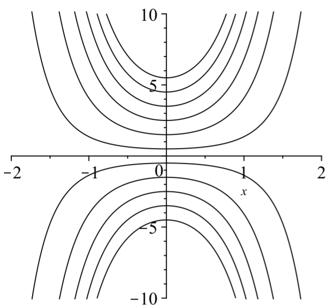
Applying \(\eqref{eq:6}\), one has \[\int \frac{d y}{y}=\int 2 x d x+C .\nonumber \] Integrating yields \[\ln |y|=x^{2}+C .\nonumber \] Exponentiating, one obtains the general solution, \[y(x)=\pm e^{x^{2}+C}=A e^{x^{2}} .\nonumber \] Here we have defined \(A=\pm e^{C}\). Since \(C\) is an arbitrary constant, \(A\) is an arbitrary constant. Several solutions in this 1-parameter family are shown in Figure \(\PageIndex{1}\).

Figure \(\PageIndex{1}\): Plots of solutions from the \(1-\)parameter family of solutions of Example \(\PageIndex{1}\) for several initial conditions.

Next, one seeks a particular solution satisfying the initial condition. For \(y(0)=\) 2 , one finds that \(A=2\). So, the particular solution satisfying the initial condition is \(y(x)=2 e^{x^{2}}\).

Example \(\PageIndex{2}\)

\(y y^{\prime}=-x\).

Solution

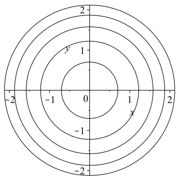
Following the same procedure as in the last example, one obtains: \[\int y d y=-\int x d x+C \Rightarrow y^{2}=-x^{2}+A, \text { where } A=2 C .\nonumber \] Thus, we obtain an implicit solution. Writing the solution as \(x^{2}+y^{2}=A\), we see that this is a family of circles for \(A>0\) and the origin for \(A=0\). Plots of some solutions in this family are shown in Figure \(\PageIndex{2}\).

Figure \(\PageIndex{2}\): Plots of solutions of Example \(\PageIndex{2}\) for several initial conditions.

Linear First Order Equations

The second type of first order equation encountered is the linear first order differential equation in the standard form \[y^{\prime}(x)+p(x) y(x)=q(x) .\label{eq:7}\] In this case one seeks an integrating factor, \(\mu(x)\), which is a function that one can multiply through the equation making the left side a perfect derivative. Thus, obtaining, \[\frac{d}{d x}[\mu(x) y(x)]=\mu(x) q(x) .\label{eq:8}\]

The integrating factor that works is \(\mu(x)=\exp \left(\int^{x} p(\xi) d \xi\right)\). One can derive \(\mu(x)\) by expanding the derivative in Equation \(\eqref{eq:8}\), \[\mu(x) y^{\prime}(x)+\mu^{\prime}(x) y(x)=\mu(x) q(x),\label{eq:9}\] and comparing this equation to the one obtained from multiplying \(\eqref{eq:7}\) by \(\mu(x)\) : \[\mu(x) y^{\prime}(x)+\mu(x) p(x) y(x)=\mu(x) q(x) .\label{eq:10}\] Note that these last two equations would be the same if the second terms were the same. Thus, we will require that \[\frac{d \mu(x)}{d x}=\mu(x) p(x) .\nonumber \] This is a separable first order equation for \(\mu(x)\) whose solution is the integrating factor: \[\mu(x)=\exp \left(\int^{x} p(\xi) d \xi\right) . \label{eq:11}\]

Equation \(\eqref{eq:8}\) is now easily integrated to obtain the general solution to the linear first order differential equation: \[y(x)=\frac{1}{\mu(x)}\left[\int^{x} \mu(\xi) q(\xi) d \xi+C\right] .\label{eq:12}\]

Example \(\PageIndex{3}\)

\(x y^{\prime}+y=x, \quad x>0, y(1)=0\).

Solution

One first notes that this is a linear first order differential equation. Solving for \(y^{\prime}\), one can see that the equation is not separable. Furthermore, it is not in the standard form \(\eqref{eq:7}\). So, we first rewrite the equation as \[\frac{d y}{d x}+\frac{1}{x} y=1 \text {. }\label{eq:13}\] Noting that \(p(x)=\frac{1}{x}\), we determine the integrating factor \[\mu(x)=\exp \left[\int^{x} \frac{d \xi}{\xi}\right]=e^{\ln x}=x .\nonumber \] Multiplying equation \(\eqref{eq:13}\) by \(\mu(x)=x\), we actually get back the original equation! In this case we have found that \(x y^{\prime}+y\) must have been the derivative of something to start. In fact, \((x y)^{\prime}=x y^{\prime}+x\). Therefore, the differential equation becomes \[(x y)^{\prime}=x .\nonumber \] Integrating, one obtains \[x y=\frac{1}{2} x^{2}+C\nonumber \] or \[y(x)=\frac{1}{2} x+\frac{C}{x} .\nonumber \]

Inserting the initial condition into this solution, we have \(0=\frac{1}{2}+C\). Therefore, \(C=-\frac{1}{2}\). Thus, the solution of the initial value problem is \[y(x)=\frac{1}{2}\left(x-\frac{1}{x}\right) .\nonumber \]

We can verify that this is the solution. Since \(y^{\prime}=\frac{1}{2}+\frac{1}{2 x^{2}}\), we have \[x y^{\prime}+y=\frac{1}{2} x+\frac{1}{2 x}+\frac{1}{2}\left(x-\frac{1}{x}\right)=x \text {. }\nonumber \] Also, \(y(1)=\frac{1}{2}(1-1)=0\).

Example \(\PageIndex{4}\)

\((\sin x) y^{\prime}+(\cos x) y=x^{2}\).

Solution

Actually, this problem is easy if you realize that the left hand side is a perfect derivative. Namely, \[\frac{d}{d x}((\sin x) y)=(\sin x) y^{\prime}+(\cos x) y .\nonumber \] But, we will go through the process of finding the integrating factor for practice.

First, we rewrite the original differential equation in standard form. We divide the equation by \(\sin x\) to obtain \[y^{\prime}+(\cot x) y=x^{2} \csc x\nonumber \] Then, we compute the integrating factor as \[\mu(x)=\exp \left(\int^{x} \cot \xi d \xi\right)=e^{\ln (\sin x)}=\sin x .\nonumber \] Using the integrating factor, the standard form equation becomes \[\frac{d}{d x}((\sin x) y)=x^{2} .\nonumber \] Integrating, we have \[y \sin x=\frac{1}{3} x^{3}+C\nonumber \] So, the solution is \[y(x)=\left(\frac{1}{3} x^{3}+C\right) \csc x .\nonumber \]