
1.4: Predictor-corrector methods and Runge-Kutta
- Page ID
- 108071

Heun’s method
The next ODE solver is Heun’s method. It uses a new approach to computing the best step to take from the current position \((t_n, y_n)\). To better appreciate Heun’s method, let’s first review the problems experienced by the two methods studied so far:
- Forward Euler. In forward Euler we compute the slope of \(y(t)\) at the current time \(t_n\) and use that slope to take a step forward into the future. The problem with forward Euler is that the function \(f(t, y)\) might curve away from the line predicted by the slope at \(t_n\). Consequently, forward Euler’s accuracy is \(O(h)\) – which is low.
- Backward Euler. Backward Euler uses the slope at time \(t_{n+1}\) to compute the forward step. Once again, however, the solution \(y(t)\) can curve away from the line predicted by the slope at \(t_{n+1}\), so the accuracy is again low.
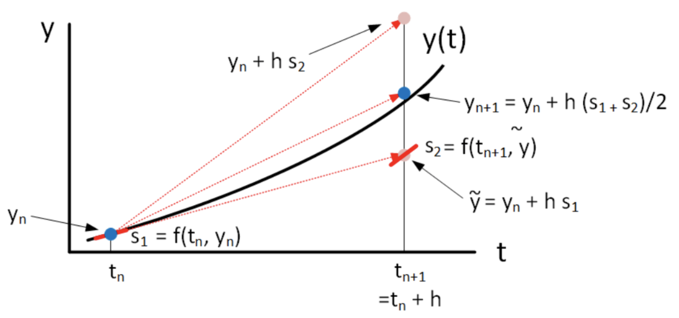
The problem with both methods is that they use a linear approximation to the behavior of the solution inside the interval \(t_n \le t \le t_{n+1}\), and use a slope computed at the end of the interval. Heun’s method tries to fix this problem by retaining the linear approximation, but averaging the slopes from both ends of the domain. Specifically, Heun’s method does the following:
- Sit at \(t=t_n\) and compute the slope at this point, \(s_1 = f(t_n, y_n)\).
- Use this slope to estimate the solution’s value at \(t_{n+1}\) using standard forward Euler: \(\tilde{y}(t_{n+1}) = y(t_n) + h f(t_n, y_n)\). Note we denote this point \(\tilde{y}(t_{n+1})\) using a tilde \(\sim\) since it’s an intermediate step towards our solution.
- At this point \((t_n, \tilde{y}_{n+1})\) compute the slope \(s_2 = f(t_{n+1}, \tilde{y}_{n+1})\).
- Average these two slopes to compute the forward step: \[\tag{eq:4.1} y(t_{n+1} ) = y(t_n) + \frac{h}{2} \left( s_1 + s_2 ) \right)\]
The method still assumes a straight-line approximation to \(y(t)\) in the interval \(t_n \le t \le t_{n+1}\) but uses a better approximation to the slope. The formal algorithm is presented in [alg:4]. This process is shown graphically in 4.1.
__________________________________________________________________________________________________________________________________
Algorithm 4 Heun's method
__________________________________________________________________________________________________________________________________
Inputs: initial condition \(y_0\), end time \(t_{end}\).
Initialize: \(t_0 = 0, y_0\).
for \(n=0: t_{end}/h\) do
Compute slope at \(t_n\): \(S_1 \leftarrow f(t_n, y_n)\)
Compute intermediate step at \(t_{n+1}\): \(\tilde{y} \leftarrow y_n + h S_1\)
Compute slope at \(t_{n+1}\): \(S_2 \leftarrow f(t_{n+1}, \tilde{y})\)
Compute final step: \(y_{n+1} \leftarrow y_n + (h/2)(S_1 + S_2)\)
end for
return \(y\) vector.
__________________________________________________________________________________________________________________________________
The plot shows the result of computing \(y_{n+1}\) using forward and backward Euler as well as Heun’s method. The thing to observe is that for the function curvature shown, forward Euler undershoots the actual function value at \(y_{n+1}\) and backward Euler overshoots it. However, since Heun’s method averages the present and (guessed) future slopes, it comes much closer to hitting the desired correct value of \(y_{n+1}\).
Heun’s method is perhaps the most basic ODE solver in a large family of solvers which are called "predictor-corrector" methods. The idea is that these methods first take one or more "predictor" steps into the future, then use the results of the predictor steps to compute the "corrector" – the actual step. In the case of Heun’s method we have:
- Predictor: \(\tilde{y} = y_n + h f(t_n, y_n)\)
- Corrector: \(y_{n+1} = y_n + (h/2)(f(t_n, y_n) + f(t_{n+1}, \tilde{y}))\)
In some sense, these intermediate \(y\) values are used to "feel" what the slope looks in the future. Once enough trial steps have been taken (predictor step), then they are combined together (corrector step) to form the final step.
Example: the exponential growth ODE and error scaling
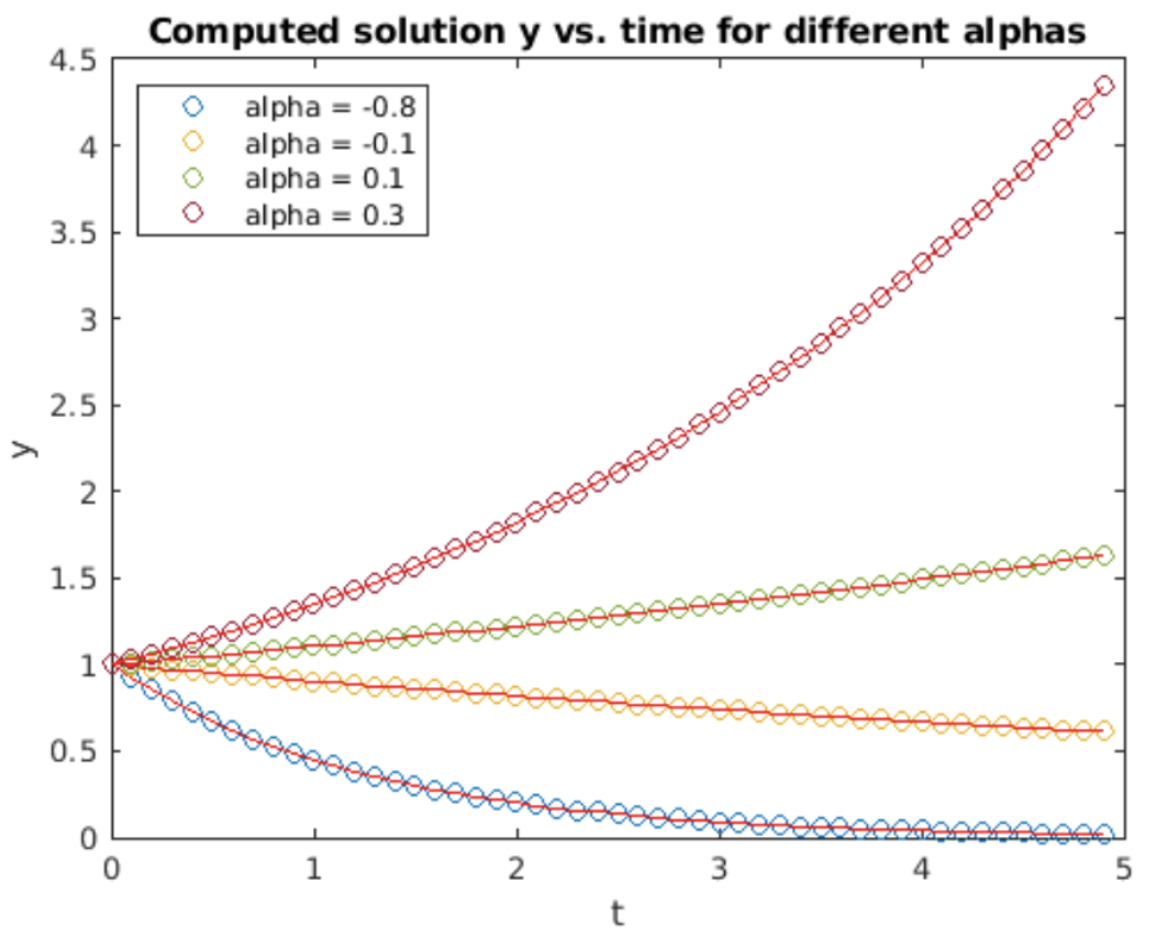
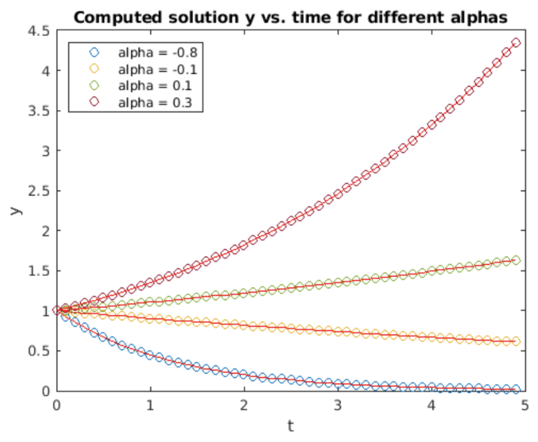
As usual, we examine the result of using Heun’s method on the exponential growth ODE, [eq:2.5]. Simulation results are shown in fig. 4.2. The computed solution clearly gives a better match to the analytic results – Heun’s method is a better method than forward Euler!
We can quantify the accuracy of Heun’s method by computing the RMS error between the computed and the analytic solutions for different stepsizes \(h\). This is shown in 4.3. On a log-log plot the slope of the error line is two – the order of Heun’s method is accordingly \(O(h^2)\). That is, if we halve the stepsize then we get a factor of four improvement in method accuracy. This is much better than the \(O(h)\) accuracy offered by forward Euler.

Example: the simple harmonic oscillator
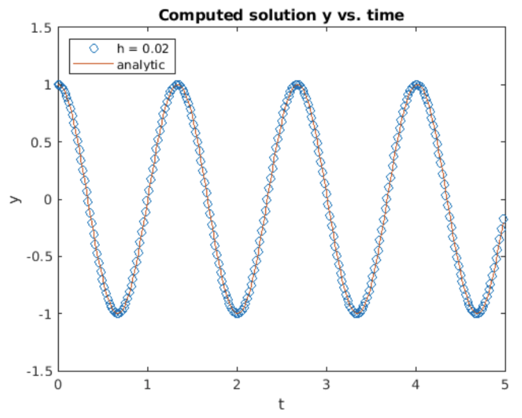
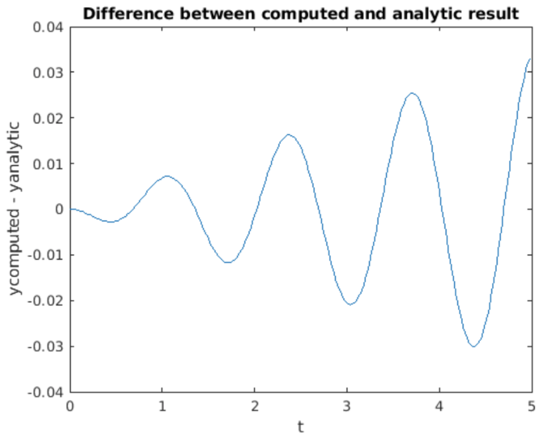
Our friend the simple harmonic oscillator is also easy to implement using Heun’s method. The result of running Heun’s method using a larger step size than used for both forward and backward Euler is shown in 4.4. Compared to both forward and backward Euler, the oscillation neither grows nor decays significantly over the 5 second simulation time – at least on the scale of 4.4. This suggests Heun’s method is a superior algorithm to both forward and backward Euler. The better accuracy is a result of using slope information from both time \(t_n\) as well as \(t_{n+1}\) – this gives the method an \(h^2\) order. Nonetheless, all is not rosy – see 4.5 which plots the difference between the computed and the analytic solution. The difference evidently grows exponentially, although the magnitude is not as bad as with the Euler methods.
Midpoint method
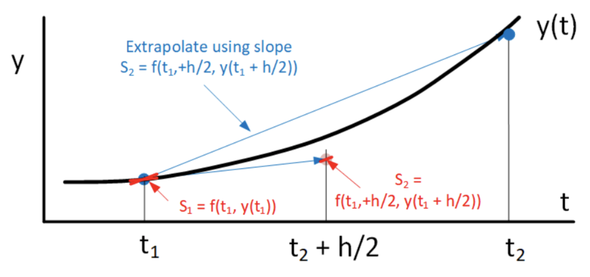
A similar method to Heun’s is the midpoint method. We will specifically look at the explicit midpoint method (there is also an implicit midpoint method). The midpoint method uses forward Euler to take a half-step forward, then computes the slope at that point and uses that slope to make the full step. The algorithm is presented in [alg:5]. A drawing showing how the midpoint method works is shown in 4.6.
__________________________________________________________________________________________________________________________________
Algorithm 5 Midpoint method
__________________________________________________________________________________________________________________________________
Inputs: initial condition \(y_0\), end time \(t_{end}\).
Initialize: \(t_0 = 0, y_0\).
for \(n=0: t_{end}/h\) do
Compute slope at \(t_n\): \(s_1 \leftarrow f(t_n, y_n)\)
Compute intermediate step to \(t_{n} + h/2\): \(\tilde{y} \leftarrow y_n + (h/2) s_1\)
Compute slope at \(t_{n} + h/2\): \(s_2 \leftarrow f(t_{n}+h/2, \tilde{y})\)
Compute final step: \(y_{n+1} \leftarrow y_n + h s_2\)
end for
return \(y\) vector.
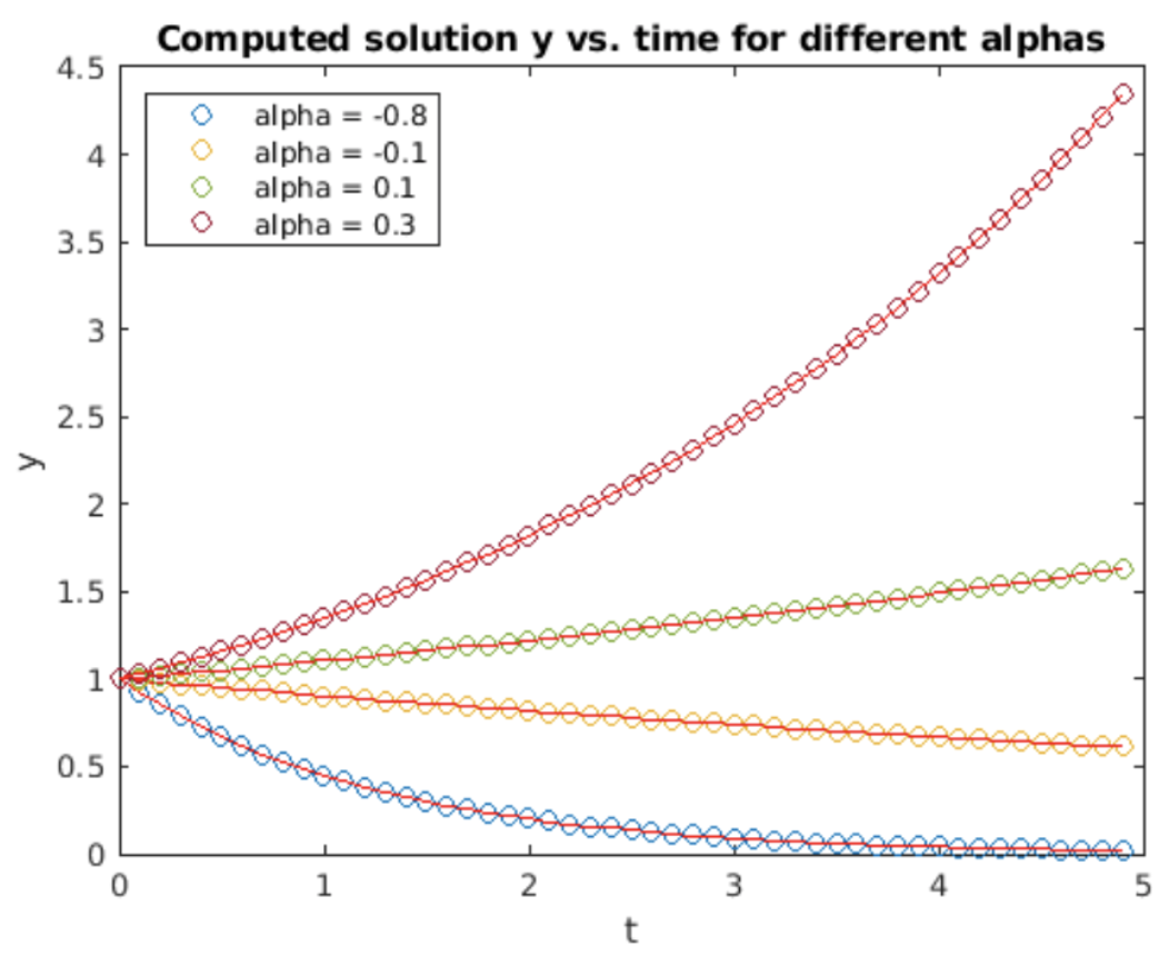
Example: the exponential growth ODE
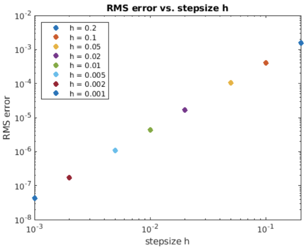
We examine the midpoint method on the exponential growth ODE, [eq:2.5]. Simulation results are shown in 4.7. The computed solution clearly gives a better match to the analytic results than forward Euler – the midpoint method is also a better method than forward Euler! The RMS error vs. stepsize plot is shown in 4.8. On a log-log plot the slope of the error line is two – this says that the order of the method is \(O(h^2)\).
Runge-Kutta methods
The most famous predictor-corrector methods are the Runge-Kutta methods. Even if you have had only passing familiarity with numerical methods for ODEs in the past, you have probably heard of these methods, or even used them! In particular, 4th-order Runge-Kutta is the most common workhorse used when solving ODEs. It is the go-to solver used to solve the majority of ODEs. A variant of 4th-order Runge-Kutta is built into Matlab as the function ode45. There are plenty of other ODE solvers available, but one generally tries 4th order Runge-Kutta first, and if it doesn’t work or produces poor results then one turns to other, more specialized methods.
We will concentrate on the classic 4th order Runge-Kutta method since it is the most common one. Runge-Kutta methods of other orders also exist, but this 4th order method is both most common and also shows all the relevant concepts you should learn. In any event, you will likely call a pre-written solver from a library in your real work, so the important thing to learn are the concepts involved, not the details of each and every variant in the Runge-Kutta family.
In what follows we will call this particular variant of 4th order Runge Kutta "RK4" for brevity. RK4 takes four samples of the present and future slopes. Here is the method: \[\begin{aligned} \nonumber k_1 &= h f(t_n, y_n) \\ \nonumber k_2 &= h f(t_n+h/2, y_n + k_1/2) \\ \nonumber k_3 &= h f(t_n+h/2, y_n + k_2/2) \\ \nonumber k_4 &= h f(t_n+h, y_n + k_3) \\ \nonumber y_{n+1} &= y_n + (k_1 + 2 k_2 + 2 k_3 + k_4)/6\end{aligned}\] Things to note about RK4:
- RK4 computes four intermediate results, \(k_1\), \(k_2\), \(k_3\), \(k_4\). Each intermediate result relies on the preceeding computation – that means you must perform the computations in order. The computation is depicted graphically in 4.9.
- The final result is a weighted sum of the intermediate results.
- RK4 is an explicit method – no rootfinding is required to compute the desired result.
- You might wonder where the sample points and the coefficients in the weighted sum come from. The short answer is, they are something you look up in a book (or online). The longer answer is, of course they may be derived, but the derivation is long and tedious and doesn’t lend any insight into the method. Therefore, we will skip the derivation here.
- We have depicted \(y\) to be a scalar in the above – that is, we assumed we are solving a single, scalar ODE. However, just as in the previous methods, \(y\) may also be a vector – that is, RK4 may also be used to solve a system of ODEs in the same way as may be used for all previous methods.

Example: the exponential growth ODE
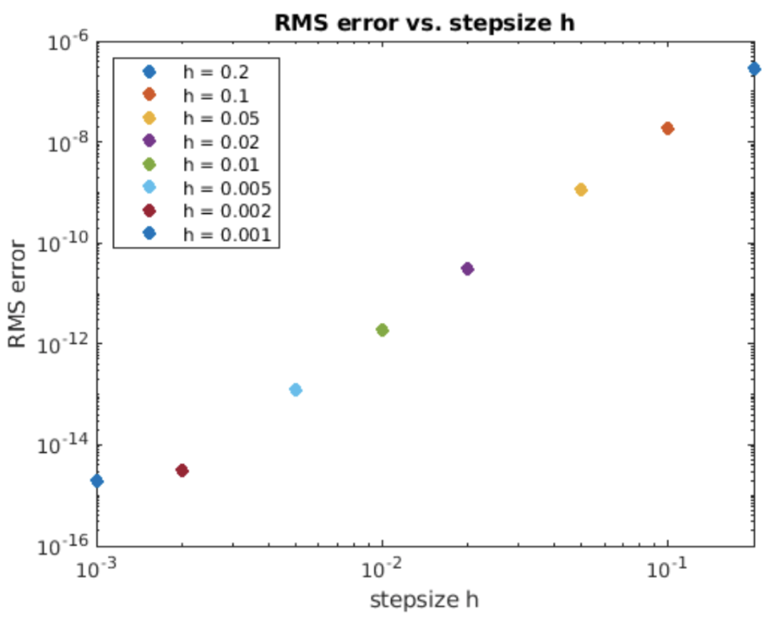
We examine using RK4 on the usual exponential growth ODE, [eq:2.5]. Simulation results are shown in 4.10. The computed solution matches the analytic result closely. The RMS error vs. stepsize plot is shown in 4.11. This time the slope on a log-log plot is four – this says that the order of the method is \(O(h^4)\).
Example: the simple harmonic oscillator
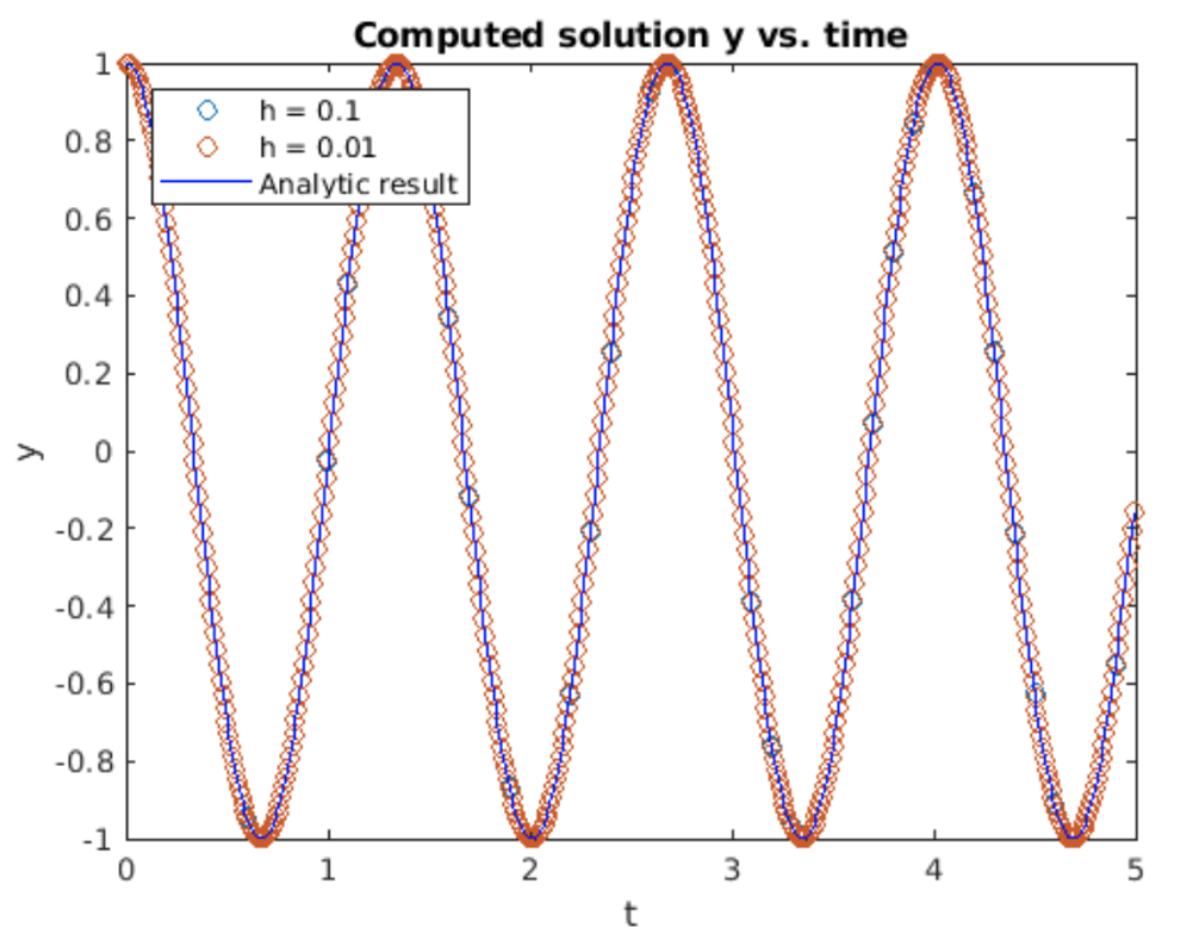
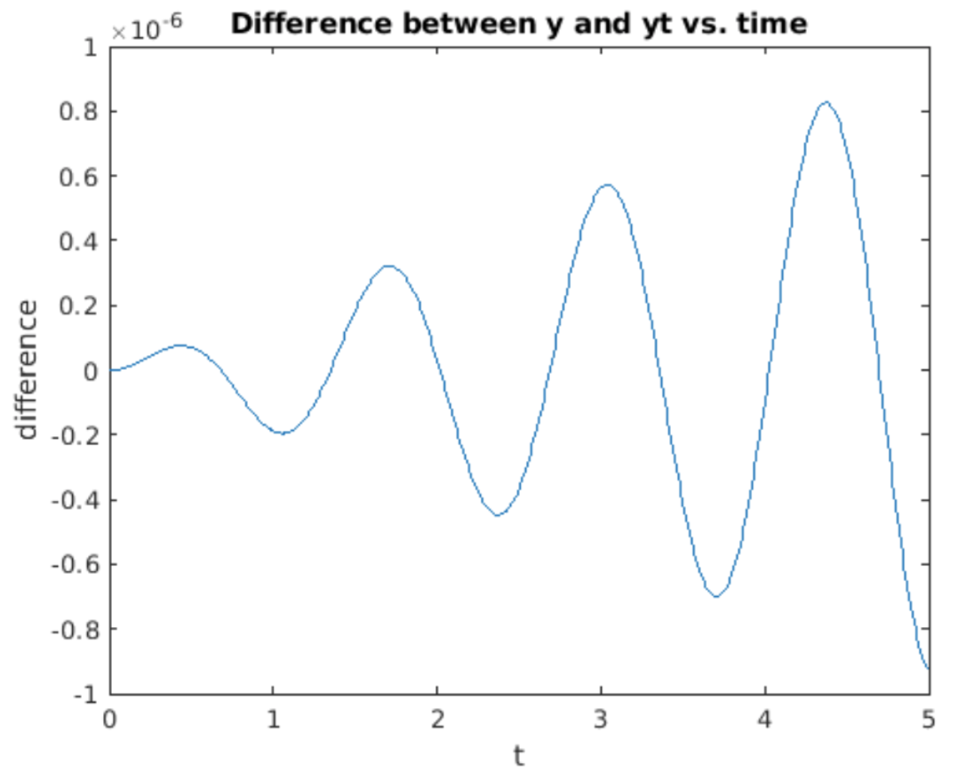
Let’s explore using RK4 using our old friend the SHO. Once again broken down into two first order ODEs, the SHO is \[\begin{aligned} \nonumber \frac{d u}{d t} &= -\frac{k}{m} v \\ \nonumber \frac{d v}{d t} &= u\end{aligned}\] To use RK4 we write this in the general form \[\begin{aligned} \frac{d u}{d t} &= f(t, u, v) \\ \frac{d v}{d t} &= g(t, u, v) \end{aligned} \tag{eq:4.2}\] with \(f(t, u, v) = -(k/m) v\) and \(g(t, u, v) = u\). To implement this method on the computer we treat all variables as vectors. That is, we gather the LHS expression as \[\nonumber y = \begin{pmatrix} du/dt \\ dv/dt \end{pmatrix}\] and the RHS as \[\nonumber F = \begin{pmatrix} f(t, u, v) \\ g(t, u, v) \end{pmatrix}\] so the vectorized system to integrate is \[\nonumber \frac{dy}{dt} = F(t, y)\] Then each of the intermediate steps \(k_i\) is a \(2 \times 1\) column vector. Writing the problem this way makes it easy to implement RK4 using vectorized expressions. Results obtained for integrating the SHO using RK4 are shown in 4.12 alongside the analytic result \(\cos(\omega t)\). The results look great – both \(h = 0.1\) and \(h=0.01\) produce cosine waves which look picture-perfect – at least over the scale and time period simulated. However, the results are not perfect – 4.13 shows the difference (error) between the computed and the analytic results. Although the difference is small, it is nonzero. Worse, the error grows exponentially with increasing time. This suggests the RK4 method – like forward and backward Euler – is unstable for the simple harmonic oscillator, albeit much better than the other methods.
Example: the hanging pendulum
We have employed the simple harmonic oscillator as a useful example to demonstrate the different solvers encountered so far. The SHO is sometimes used as a linearized model of the motion of a hanging pendulum. However, a real hanging pendulum’s motion is governed by a nonlinear ODE. The geometry of the problem is shown in 4.14.
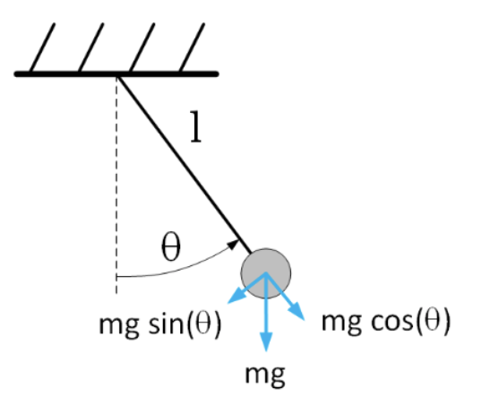
The independent variable is time \(t\), the dependent variable (which we want to solve for) is the angle \(\theta\) made by the pendulum with respect to vertical. The pendulum’s length is \(l\) and the gravitational force constant is \(g\). The ODE is derived as follows:
- We consider the forces acting on the pendulum when it is displaced from the vertical by an angle \(\theta\). In particular, gravity pulls the pendulum down with a constant vertical force \(m g\).
- The vertical force may be resolved into two components: One in the \(\hat{r}\) direction – in line with the pendulum’s support, and one in the \(\hat{\theta}\) direction. Elementary trig says the force in the \(\hat{\theta}\) direction is \(F_{\theta} = -m g \sin(\theta)\). The negative sign appears since the force pulls the pendulum bob back to the equilibrium point at \(\theta = 0\).
- Newton’s second law states \(F = m a\). In the case of the pendulum bob, \(F\) is the force acting in the \(\hat{\theta}\) direction, and \(a\) is the acceleration in the \(\hat{\theta}\) direction. Since the pendulum bob is attached to the rod of length \(l\), the angular acceleration is \(l d^2 \theta / d t^2\).
- Using the above information, the equation governing the pendulum’s motion is \[\nonumber m l \frac{d^2 \theta}{d t^2} = -m g \sin(\theta)\] or \[\tag{eq:4.3} \frac{d^2 \theta}{d t^2} = -\frac{g}{l} \sin(\theta)\]
Observe that for small \(\theta\) we may approximate \(\sin(\theta) \approx \theta\) which gives back the SHO. But for large pendulum swings this approximation doesn’t work and we need to use the full, non-linear expression for the restoring force on the pendulum bob. In this case an analytic solution for [eq:4.3] exists – the analytic solution may be expressed using the Jacobi elliptic functions sn and cn. However, rather than playing around with higher transcendental functions, we’ll just use RK4 to compute the solutions numerically.
To proceed, we break the second order ODE [eq:4.3] into two first order ODEs. We get \[\begin{aligned} \nonumber \frac{du}{dt} &= v \\ \nonumber \frac{dv}{dt} &= -\frac{g}{l} \sin(u)\end{aligned} \label{eq:NonlinearPendEqTwoODEs}\] Now we rearrange this system into a vector form for use with the Runge-Kutta implementation. We get \[\begin{aligned} \begin{pmatrix} du/dt \\ dv/dt \end{pmatrix} = \begin{pmatrix} v \\ -(g/l) \sin(u) \end{pmatrix} \end{aligned} \tag{eq:4.4}\] This form is ready for implementation. The vectorized form [eq:4.4] is implemented in a function called by the RK4 integrator itself, and a test wrapper is the main program run by the user. This is the usual software architecture previously shown in 2.2.
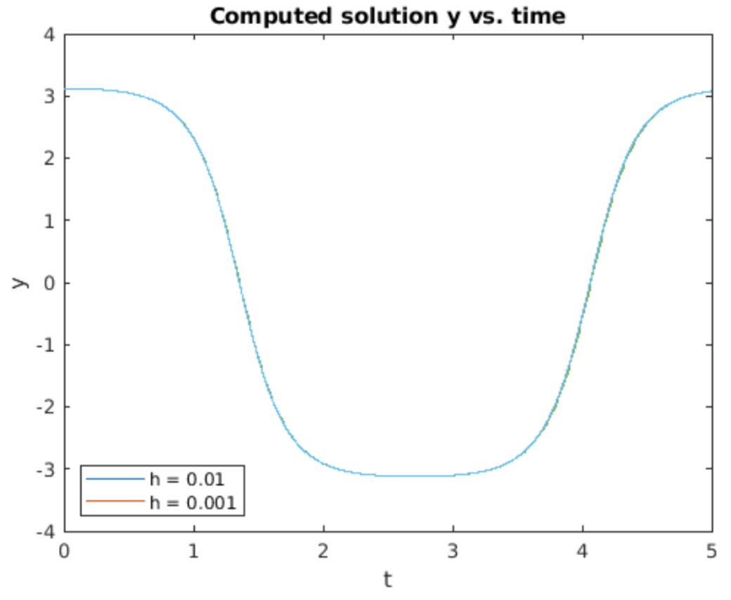
Running the RK4 implementation gives the plot shown in 4.15. This plot was obtained using \(g = 9.8\) m/sec\(^2\) (the value of \(g\) at the earth’s surface) and \(l = 0.5\)m, a reasonable value for the length of a pendulum. For initial conditions, the pendulum swing started with the bob pointing almost vertically up. Therefore, the pendulum takes a long time for the bob to accelerate. It then swings quickly around the downward hanging position and continues until pointing almost vertically up again. The pendulum then repeats this motion again and again, never stopping because the original equation does not include any dissipation (friction).
Example: the Van der Pol oscillator
In the 1920, the Dutch physicist Balthasar van der Pol was employed by Philips to work on vacuum tubes. Vacuum tubes were electronic devices used to amplify signals in the days before transistors. Van der Pol found that under certain circumstances the vacuum tubes would spontaneously oscillate on their own. Uncontrolled self-oscillations are a very undesirable behavior, so he was interested in understanding why they happened. Van der Pol investigated the physical reasons for the oscillation and determined that the voltage swing across the vacuum tube could be modeled by the second order ODE \[\tag{eq:4.5} \frac{d^2 y}{d t^2} - \epsilon(1 - y^2)\frac{d y}{d t} + y = 0\] where \(y\) is the voltage across the tube. The \(\epsilon\) term represents a non-linear damping since it involves the \(d y/d t\) term. When \(y < 1\) this term represents amplification: it imparts a positive value to \({d^2 y}/{d t^2}\) when \({d y}/{d t}\) is also positive, thereby the amplitude of the oscillation increases. When \(y > 1\) the opposite happens: the term adds a negative value to \({d^2 y}/{d t^2}\) for positive \({d y}/{d t}\) causing the amplitude of the oscillation to decrease. Therefore, the action of the \(\epsilon\) term is to create an oscillation whose amplitude remains bounded in time.
This second order ODE may be broken into two first order ODEs by defining \[\begin{aligned} \nonumber u &= y \\ \nonumber v &= \frac{d y}{d t}\end{aligned}\] Then, the ODE system is \[\begin{aligned} \label{eq:VanDerPolOscSystem} \nonumber \frac{d u}{d t } &= v \\ \nonumber \frac{d v}{d t} &= \epsilon(1 - u^2) v - u\end{aligned}\]
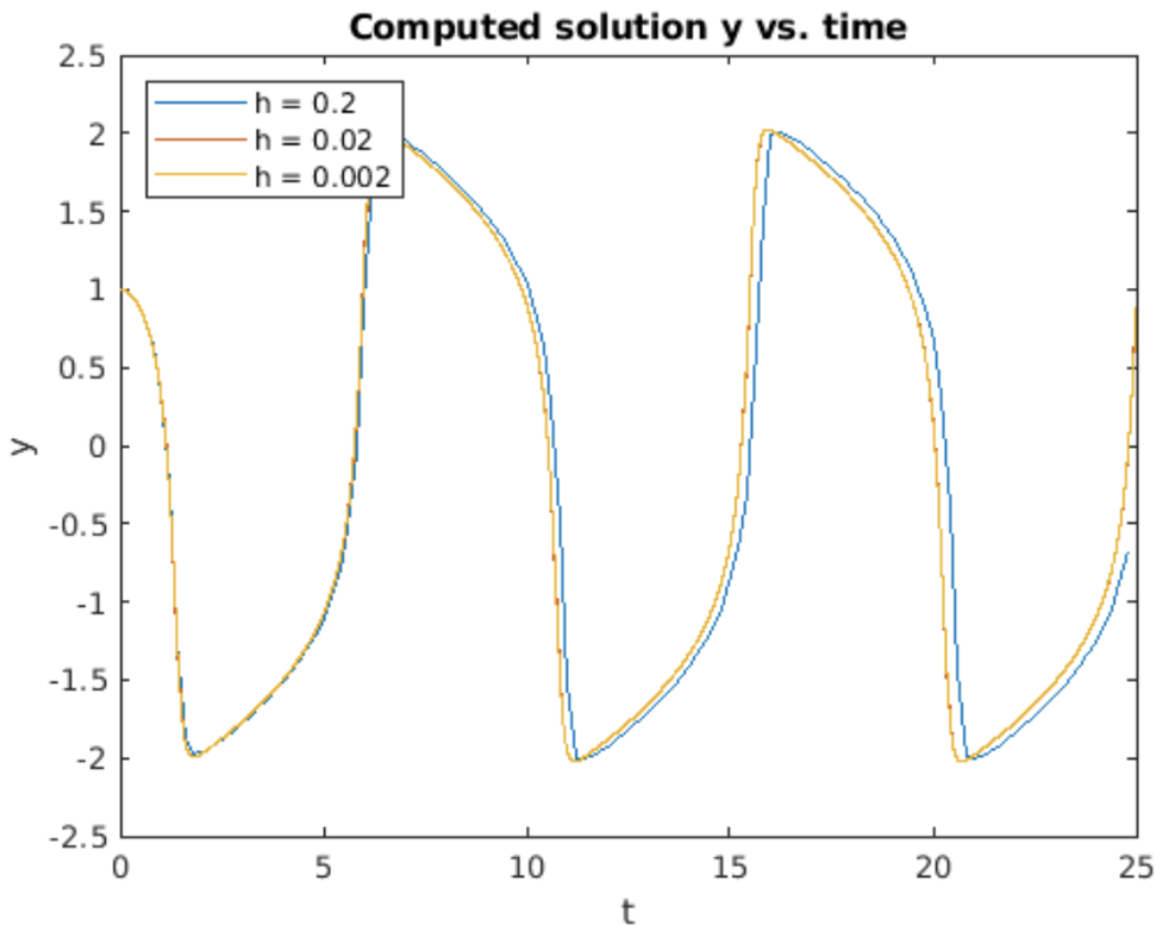
Integrating this system using RK4 gives the plot shown in 4.16. Things to note about the results shown in 4.16:
- As predicted, after a quick start-up phase, the Van der Pol ODE produces a constant amplitude, periodic oscillation. We note that the oscillation looks nothing like the usual sin or cosine oscillations produced by linear oscillators. The strong nonlinearity introduced by the \(dy/dt\) term is the reason for behind this shape.
- Note that the \(h=0.2\) curve is displaced from the curves generated with smaller \(h\) values. This is a real effect. is a so-called "stiff" ODE, which makes it difficult to solve numerically, at least using larger step sizes. This property will be detailed in section 5.3 below.
Example: Duffing’s equation
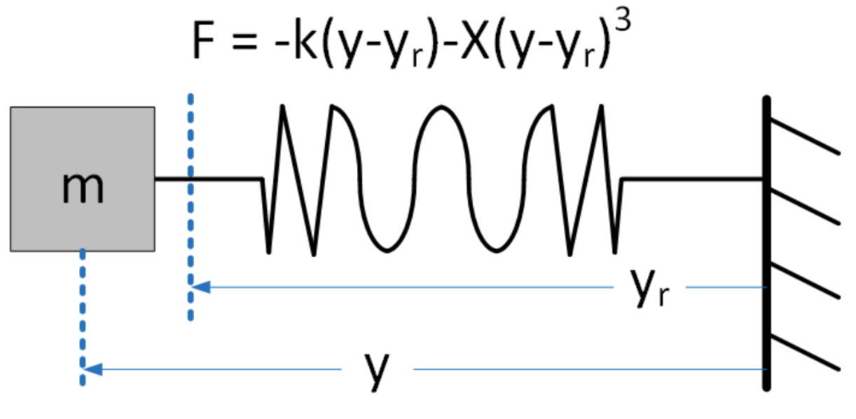
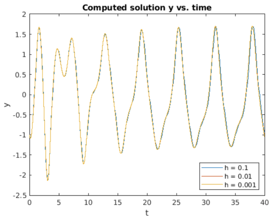
Duffing’s equation is a nonlinear variant of the simple harmonic oscillator. It models the situation where the spring’s response is not linear for all extensions, but rather the spring’s restoring force grows faster than linearly at the ends of the spring’s travel. This models the real-world behavior of springs – springs don’t behave linearly if you pull on the spring to the end of it’s extent. Duffing’s equation models the stiffness by adding a cubic term to the restoring force. For small displacements the cubic force is small, but for larger displacements it will dominate the return force. On the RHS, Duffing also adds a drive force – in this case a cosine drive of frequency \(\omega\). A drawing of the physical setup is shown in 4.17. The full Duffing’s equation is \[\tag{eq:4.6} \frac{d^2 y}{d t^2} + \delta \frac{d y}{d t} + \alpha y + \beta y^3 = \gamma \cos(\omega t)\]
Butcher tableaux
As mentioned above, there are many different variants of the Runge-Kutta method itself, as well as other types of predictor-corrector methods. A useful device which catalogs the different methods are the Butcher tableaux. These are tables summarizing the different coefficients which make up a particular method. A general, explicit predictor-corrector method looks like this: \[\begin{aligned} k_1 =& h f(t_n, y_n) \\ k_2 =& h f(t_n + c_2 h, y_n + a_{21} k_1) \\ k_3 =& h f(t_n + c_3 h, y_n + a_{31} k_1 + k_{32} k_2) \\ & \vdots \\ y_{n+1} =& y_n + \left( b_1 k_1 + b_2 k_2 + b_3 k_3 + \cdots \right) \end{aligned} \tag{eq:4.7}\] Compare this to the definition of RK4 shown above. A Butcher tableau summarizes the coefficients as shown the [tab:4.1].
| \(c_1\) | \(a_{11}\) | \(a_{12}\) | \(a_{13}\) | \(\cdots\) |
| \(c_2\) | \(a_{21}\) | \(a_{22}\) | \(a_{23}\) | \(\cdots\) |
| \(c_3\) | \(a_{31}\) | \(a_{32}\) | \(a_{33}\) | \(\cdots\) |
| \(\vdots\) | \(\vdots\) | \(\vdots\) | \(\vdots\) | \(\ddots\) |
| \(b_1\) | \(b_2\) | \(b_3\) | \(\cdots\) |
As examples, Butcher tableaux for Heun’s method, the midpoint method, and RK4 are shown in [tab:4.2] - [tab:4.4]. Compare the coefficients in the tables against the definitions of the solver methods to see how they are related.
| 0 | 0 | 0 |
| 1 | 1 | 0 |
| 1/2 | 1/2 |
\[\begin{aligned} \nonumber k_1 &= h f(t_n, y_n) \\ \nonumber k_2 &= h f(t_n+h, y_n + k_1) \\ \nonumber y_{n+1} &= y_n + k_1/2 + k_2/2 \end{aligned}\]
Table 4.2: Heun's method
| 0 | 0 | 0 |
| 1/2 | 1/2 | 0 |
| 0 | 1 |
\[\begin{aligned} \nonumber k_1 &= h f(t_n, y_n) \\ \nonumber k_2 &= h f(t_n+h/2, y_n + k_1/2) \\ \nonumber y_{n+1} &= y_n + k_2 \end{aligned}\]
Table 4.3: Midpoint method
| 0 | 0 | 0 | 0 | 0 |
| 1/2 | 1/2 | 0 | 0 | 0 |
| 1/2 | 0 | 1/2 | 0 | 0 |
| 1 | 0 | 0 | 1 | 0 |
| 1/6 | 1/3 | 1/3 | 1/6 |
\[\begin{aligned} \nonumber k_1 &= h f(t_n, y_n) \\ \nonumber k_2 &= h f(t_n+h/2, y_n + k_1/2) \\ \nonumber k_3 &= h f(t_n+h/2, y_n + k_2/2) \\ \nonumber k_4 &= h f(t_n+h, y_n + k_3) \\ \nonumber y_{n+1} &= y_n + (k_1 + 2 k_2 + 2 k_3 + k_4)/6 \end{aligned}\]
Table 4.4: Fourth-order Runge-Kutta
Chapter summary
Here are the important points made in this chapter:
- Predictor-corrector methods "feel" the slope at different times in the future in order to compute the best step forward in time.
- Heun’s method and the midpoint method are simple examples of predictor-corrector methods. Both are \(O(h^2)\) methods.
- The workhorse method used to solve a large fraction of ODEs in the world is 4th order Runge-Kutta. This method is the first thing you should try when faced with a new ODE if you don’t have any special knowledge about the ODE’s properties.
- As you might expect from its name, the RMS error of 4th order Runge-Kutta scales as \(O(h^4)\).
- All methods shown in this chapter are explicit.
- Butcher tableaux are used to catalog the many different predictor-corrector methods by presenting their coefficients in a tabular form.