4.1: Heun’s method

The next ODE solver is Heun’s method. It uses a new approach to computing the best step to take from the current position \((t_n, y_n)\). To better appreciate Heun’s method, let’s first review the problems experienced by the two methods studied so far:

• Forward Euler. In forward Euler we compute the slope of \(y(t)\) at the current time \(t_n\) and use that slope to take a step forward into the future. The problem with forward Euler is that the function \(f(t, y)\) might curve away from the line predicted by the slope at \(t_n\). Consequently, forward Euler’s accuracy is \(O(h)\) – which is low.
• Backward Euler. Backward Euler uses the slope at time \(t_{n+1}\) to compute the forward step. Once again, however, the solution \(y(t)\) can curve away from the line predicted by the slope at \(t_{n+1}\), so the accuracy is again low.

The problem with both methods is that they use a linear approximation to the behavior of the solution inside the interval \(t_n \le t \le t_{n+1}\), and use a slope computed at the end of the interval. Heun’s method tries to fix this problem by retaining the linear approximation, but averaging the slopes from both ends of the domain. Specifically, Heun’s method does the following:

1. Sit at \(t=t_n\) and compute the slope at this point, \(s_1 = f(t_n, y_n)\).
2. Use this slope to estimate the solution’s value at \(t_{n+1}\) using standard forward Euler: \(\tilde{y}(t_{n+1}) = y(t_n) + h f(t_n, y_n)\). Note we denote this point \(\tilde{y}(t_{n+1})\) using a tilde \(\sim\) since it’s an intermediate step towards our solution.
3. At this point \((t_n, \tilde{y}_{n+1})\) compute the slope \(s_2 = f(t_{n+1}, \tilde{y}_{n+1})\).
4. Average these two slopes to compute the forward step:

   \[ y(t_{n+1} ) = y(t_n) + \frac{h}{2} \left( s_1 + s_2 \right) \label{eq:4.1}\]

    

The method still assumes a straight-line approximation to \(y(t)\) in the interval \(t_n \le t \le t_{n+1}\) but uses a better approximation to the slope. The formal algorithm is presented in [alg:4]. This process is shown graphically in 4.1.

Algorithm 4: Heun's method

Inputs: initial condition \(y_0\), end time \(t_{end}\).

Initialize: \(t_0 = 0, y_0\).

for \(n=0: t_{end}/h\) do

Compute slope at \(t_n\): \(S_1 \leftarrow f(t_n, y_n)\)

Compute intermediate step at \(t_{n+1}\): \(\tilde{y} \leftarrow y_n + h S_1\)

Compute slope at \(t_{n+1}\): \(S_2 \leftarrow f(t_{n+1}, \tilde{y})\)

Compute final step: \(y_{n+1} \leftarrow y_n + (h/2)(S_1 + S_2)\)

end for

return \(y\) vector

Figure 4.1: Heun’s method first computes an intermediate value at \(t_{n+1}\) which we call \(\tilde{y}\) using forward Euler. It then uses this value to compute the slope at \(t_{n+1}\). It then averages the two slopes at \(t_n\) and \(t_{n+1}\) to compute the actual step.

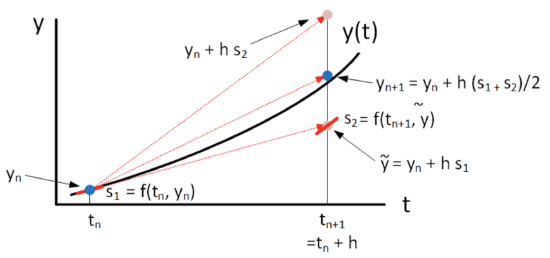
The plot shows the result of computing \(y_{n+1}\) using forward and backward Euler as well as Heun’s method. The thing to observe is that for the function curvature shown, forward Euler undershoots the actual function value at \(y_{n+1}\) and backward Euler overshoots it. However, since Heun’s method averages the present and (guessed) future slopes, it comes much closer to hitting the desired correct value of \(y_{n+1}\).

Heun’s method is perhaps the most basic ODE solver in a large family of solvers which are called "predictor-corrector" methods. The idea is that these methods first take one or more "predictor" steps into the future, then use the results of the predictor steps to compute the "corrector" – the actual step. In the case of Heun’s method we have:

• Predictor: \(\tilde{y} = y_n + h f(t_n, y_n)\)
• Corrector: \(y_{n+1} = y_n + (h/2)(f(t_n, y_n) + f(t_{n+1}, \tilde{y}))\)

In some sense, these intermediate \(y\) values are used to "feel" what the slope looks in the future. Once enough trial steps have been taken (predictor step), then they are combined together (corrector step) to form the final step.